Examples#
Let’s start with a minimal example that demonstrates how to quickly load and solve for the optimal value function and policy of a Markov Decision Process (MDP) using madupite.
We define an MDP as a tuple \((\mathcal{S}, \mathcal{A}, P, g, \gamma)\), where:
\(\mathcal{S} = \{0, 1, \dots, n-1\}\) is the set of states,
\(\mathcal{A} = \{0, 1, \dots, m-1\}\) is the set of actions,
\(P : \mathcal{S} \times \mathcal{A} \times \mathcal{S} \to [0, 1]\) is the transition probability function, where \(P(s, a, s') = \text{Pr}(s_{t+1} = s' | s_t = s, a_t = a)\) and \(\sum_{s' \in \mathcal{S}} P(s, a, s') = 1\) for all \(s \in \mathcal{S}\) and \(a \in \mathcal{A}\),
\(g : \mathcal{S} \times \mathcal{A} \to \mathbb{R}\) is the stage cost function (or reward in an alternative but equivalent formulation),
\(\gamma \in (0, 1)\) is the discount factor.
Example 1#
We start with a simple example: We have an agent that lives on a periodic 1-dimensional line of length 50. At each time step, the agent has to choose between moving to the left, to the right or staying in place. The goal is to move to the state with index 42. We want to find the optimal policy that minimizes the expected number of steps to reach the goal.
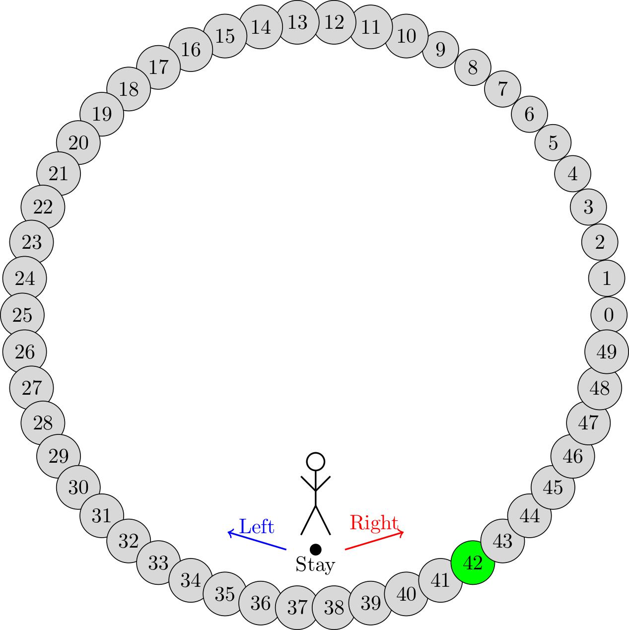
To do so, we first define the state space \(\mathcal{S} = \{0, 1, \dots, 49\}\) and the action space \(\mathcal{A} = \{0, 1, 2\}\) where 0 means staying in place, 1 means moving to the left and 2 means moving to the right.
Note that we use 0-based indexing to facilitate translating the mathematical model into code later.
For the usage in madupite, we need to provide a transition probability function that returns for a given state-action pair \((s, a)\) a list of probabilities and a list of corresponding next states. In this case, the model is deterministic and thus the probabilities are always 1. The transition probability function is defined as follows:
Stochasticity can be introduced by making the movements non-deterministic. Let’s say the when the agent moves to left or right, there is a 10% chance that they will stay in place instead. And when the agent stays in place, there is a 10% chance each that they will move to the left or right. The transition probability function is defined as follows:
Instead of defining a stage cost function, we define a reward function and set the optimization mode to maximize instead of minimize later. The reward function is defined as follows:
Turning it into code#
Let’s start by defining the transition probability function for the deterministic case:
def P_deterministic(state, action):
    if action == 0: # stay
        return [1], [state]
    if action == 1: # left
        return [1], [(state - 1) % 50]
    if action == 2: # right
        return [1], [(state + 1) % 50]
For the stochastic case:
def P_stochastic(state, action):
    if action == 0: # stay
        return [0.1, 0.8, 0.1], [(state - 1) % 50, state, (state + 1) % 50]
    if action == 1: # left
        return [0.1, 0.9], [state, (state - 1) % 50]
    if action == 2: # right
        return [0.1, 0.9], [state, (state + 1) % 50]
Next, we define the reward function:
def r(state, action):
    return 1 if state == 42 else 0
Since madupite’s distributed memory parallelism relies on MPI, it is crucial to first initialize the MPI and PETSc environment to ensure that the communication between the processes is set up correctly. This is done by creating an instance using the initialize_madupite method:
import madupite as md
instance = md.initialize_madupite()
Next we need to create the transition probability tensor and stage cost matrix using the previously defined functions. The methods createTransitionProbabilityTensor and createStageCostMatrix return a custom matrix type where the data is automaically distributed across the processes when run in parallel. Transition probability tensors are stored in a sparse format, while stage cost matrices are stored in a dense format to optimize memory usage.
For performance it is strongly recommended to preallocate the memory for the transition probability tensor as this can improve the performance of creating the objects by orders of magnitude. We refer to PETSc’s documentation for more details on how data is distributed and stored on multiple processes. The easiest (yet not the most efficient) way is to find an upper bound for the number of non-zero elements per row. That is, the maximum number of states that can be reached from a single state-action pair. For this example, this is 1 in the deterministic case and 3 in the stochastic case. Thus we create a preallocation object:
prealloc_deterministic = md.MatrixPreallocation()
prealloc_deterministic.d_nz = 1
prealloc_deterministic.o_nz = 1

prealloc_stochastic = md.MatrixPreallocation()
prealloc_stochastic.d_nz = 3
prealloc_stochastic.o_nz = 3
We refer to the PETSc documentation linked above and the madupite.MatrixPreallocation documentation in the API reference for more details on how to efficiently preallocate memory.
Finally, we create the transition probability tensor and stage cost matrix:
P_mat_deterministic = md.createTransitionProbabilityTensor(
    name="prob_ex1_deterministic",
    numStates=50,
    numActions=3,
    func=P_deterministic,
    preallocation=prealloc_deterministic
)

P_mat_stochastic = md.createTransitionProbabilityTensor(
    name="prob_ex1_stochastic",
    numStates=50,
    numActions=3,
    func=P_stochastic,
    preallocation=prealloc_stochastic
)

r_mat = md.createStageCostMatrix(
    name="reward_ex1",
    numStates=50,
    numActions=3,
    func=r
)
The functions defining the transition probabilities and stage costs / rewards will each be evaluated \(n \times m\) times in order to fill these matrices. This can be a time-consuming process why parallel execution as well as preallocation is recommended. Consider also using a JIT compiler like Numba to speed up the evaluation of these functions.
Finally we can put the ingredients together and build an MDP object:
mdp = md.MDP(instance)
mdp.setTransitionProbabilityTensor(P_mat_deterministic)
mdp.setStageCostMatrix(r_mat)
Next, we need to specify options for the solver. Two options are required for the solver to work: the discount factor \(\gamma\) and the optimization mode. The optimization mode can be either MINCOST or MAXREWARD. In this case, we defined the model as a reward maximization problem, so we set the optimization mode to MAXREWARD. The discount factor can be set to any value between 0 and 1. For this example, we set it to 0.99. See Madupite Options for a list of all available options.
mdp.setOption("-mode", "MAXREWARD")
mdp.setOption("-discount_factor", "0.99")
Finally, we can solve the MDP using the solve method:
mdp.solve()
We can re-use the same MDP object to solve the stochastic case as well. We only need to set the transition probability tensor to the stochastic one. In this case, we might also want to save the optimal policy to a file for later use:
mdp.setTransitionProbabilityTensor(P_mat_stochastic)
mdp.setOption("-file_policy", "ex1_policy.txt")
mdp.solve()
In order to run the code, save it to a file, e.g. ex1.py and run it sequentially using python ex1.py or in parallel using mpirun -n N python ex1.py where N is the number of processes.
Further examples#
Note that defining data from a function or loading from a file can be combined. See for example the maze example where the transition probabilities encode a deterministic movement in a 2D grid world and the maze logic is entirely defined in the cost function that is generated in a separate script. This can also apply to situations where e.g. costs come from measuring an experiment and are preproucessed in a separate application, independent of madupite.
Standard control applications like the double integrator and inverted pendulum using an LQR controller are also provided in the examples folder. They can also serve as examples for how to use multi-dimensional state spaces and actions.