Numerical Methods for PDEs
This page is partially complete but may still be helpful
This page attempts to concisely summarise the extensive NPDE content
Key Insights Per Chapter
We study 2nd order stationary elliptic BVPs
- The solution $u$ has the minimal energy $J(u)$
-
Elliptic similar to parabolic/hyperbolic PDEs (e.g. $\Delta u = 0$)
- $u(x): \Omega \subset \mathbb{R}^d \rightarrow \mathbb{R} $, indep. of time
1.2.1-2 Equilibrium Models
Examples of stationary elliptic BVPs (stationary/time indep.)
- String, force applied along y axis, $u$ gives displacement for every position (shape of string)
- Fixed endpoints (dirichlet BDC), $u \in C^0$ (continuous), $\Omega = [a,b]$
- Applied force $f(x)$, stiffness $\sigma$
- Get an energy $J(u)$
- Membrane, 2D version, d=2
- Electrostatic Field, $u$ is the potential at every point, dirichlet BDC on surfaces
Defined other constraints on $u$, $\Omega$, $f$, $\sigma$
- $u \in C^1_{pw}(\bar \Omega)$
- $\Omega$ bounded, $\partial \Omega$ pw smooth
- $f \in C^0_{pw}(\bar \Omega)$
- $\sigma \in C^0_{pw}(\bar \Omega)$ uniformly positive
Solution is $u = argmin_{u\in\hat V}~J(u)$, see Chp1.2.3 for all $J$’s
1.2.3 Quadratic Minimization Problems
We can rewrite all $J(u)$ as a Quadratic Functional (QF) with bi/linear forms $a(u,v)$ symmetric, $l(v)$, $u \in V_0$
- With $J: V_0 \rightarrow \mathbb{R}$
- $J(u)= {1 \over 2} a(u,u) - l(u) + c$
- $J(\eta) = {1\over 2} \eta^T A \eta - \beta^T\eta +c$, if $V_0=\R^N$ with $A\in \R^{N,N}$
- A can be found by applying unit vectors $(A)_{i,j}=a(\vec\epsilon_j, \vec\epsilon_i)$
Bi/linear see def. 0.2.1.5, for continuity see def. 1.2.3.45
By “QF = Energy Functional” and using symmetry of $a$, we can get $a$, $l$
Affine function space: $\hat V = u_0 + V_0$, $u_0$ is an offset function
- We use $u=w+u_0$ where $\hat u, u \in \hat V$ and $w \in V_0$
- note: in the tablet notes $\hat u= u + u_0$ is sometimes used
Quadratic Minimisation Problem (QMP)
- $w^* = argmin_{w \in V_0}J(w)$ with $J$ a QF
- note: $V_0$ not $\hat V$, which is why we use $w$
We can then to convert a minimisation over $u\in\hat V$ to $w\in V_0$ to get a proper QMP (see around 1.2.3.18)
- Find $u_0$ and the space $V_0$, choose $u_0$ as simple as possible, e.g. linear interpolation
- Evaluate $\tilde J(w):=J(u + u_0)$ to get $\tilde l$ and $\tilde c$ (see 1.2.3.17)
- $u = u_0 + argmin_{w \in V_0} \tilde J(w)= u_0 + w^*$
Existence & Uniqueness of a minima for a QMP
- Exists/unique $\implies$ a semi pos. def.
- $a$ pos. def. $\implies$ unique (due to convexity if $a$ p.d.)
- a s.p.d and $dim(V_0)<\infty$ $\implies$ existence and uniqueness (T1.2.3.47)
1.3 Sobolev Spaces
See ‘Norms & Spaces’
First Poincarè-Friedrichs inequality, if $\Omega \subset \mathbb{R}^d$ bounded then
- $\|u\|_0 \le diam(\Omega) \|grad(u)\|_0$, $\forall u \in H^1_0$
1.2 LVPs
$u = argmin_{v \in \hat V}J(v) \iff a(u,v)=l(v), \forall v \in V_0$
-
QMP = LVP, from $grad J(v) = 0$
-
$v$ can be considered as a perturbation function, any possible change in the minimal function $u$ will increase $J$
Terms
-
BVP (Boundary Value Problem) = PDE + BDC
-
BDC (Boundary Conditions) - Dirichlet, Neumann…
-
Quadratic functional see 1.2.3
- $J(u)= {1 \over 2} a(u,u) - l(u) + c,~~~u \in V_0$$, $ $a$ symmetric
-
QMP (Quadratic Minimisation Problem) see 1.2.3
-
LVP (Linear Variational Problem)
-
$u \in \hat V: a(u, v) = l(v), \forall v \in V_0$
-
$\hat V$ = Test Space, $V_0$ = Trial space
-
Norms & Spaces
The space to a corresponding norm is all functions $v$ s.t. $\|v\|< \infty$
- Configuration Space - set of all allowed states of a system, the range of $u$
- $S_0$ (for any $S$) functions are 0 on the boundary $\partial \Omega$
- Sometimes used to apply homogeneous Dirichlet BDC
- Affine fct. space, $u_0$ is an offset fct.
- $\hat V = u_0 + V_0$
- Energy Norm to a corresponding bilinear form $a$
- $\|v\|_a=a(v,v)^{1\over2}$
- L2 Norm, ~ average function value
- $\|v\|_{L^2(\Omega)} = \|v\|_0 = (\int |v(x)|^2 dx)^{1 \over 2}$
- $C^0_{pw} \subset L^2$
- Cannot impose Dirichlet boundary conditions
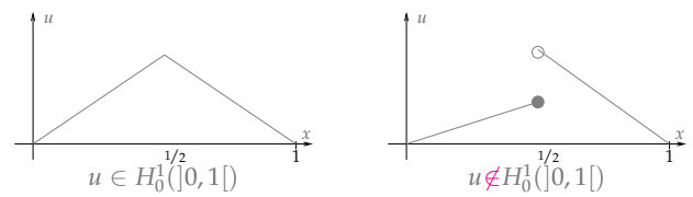
- H1 Norm, ~ average function gradient
- $\|v\|_{H^1(\Omega)} = \|v\|_1= \|v\|_0 + |v|_{H1}$
- $|v|_1 = (\int \|grad (v)\|^2 dx)^{1 \over 2}$
- Note: $u \in H^1 \implies u \in L^2$
- $C^1_{pw} \subset H^1$ so
- $H^1_*$ = $H^1_0$ where mean function value is 0
- i.e. ${v \in H^1_0 : \int v~dx = 0}$
Extra
- Stationary $\iff$ time independent