Computational Thinking (Python)

Overview

Here is a cheat sheet for python.

This course provides a comprehensive overview of the key topics in computer science, filling in the knowledge gaps between Information Technology & EE and the Computer Science bachelor's degrees. It is designed to provide students with a comprehensive understanding of the key topics in computer science and to prepare them for advanced studies in various computer science fields. This course uses Python for code examples. The curriculum covers seven critical areas of study including:

1. Algorithms: In this section, the fundamental concepts of algorithms are explored, including recursive, greedy, backtracking, dynamic programming, linear programming, linear relaxation, and flow algorithms.




2. Complexity Theory: This section covers the complexity topics of P and NP, NP-hard, Boolean Formulas and Circuits, solving hard problems, approximation techniques for vertex cover, bin packing, metric (Travelling Salesman Problem)TSP and knapsack, and the non-approximability of TSP.




3. Cryptography: This section covers various topics including encryption techniques such as perfect encryption, key exchange protocals, public key cryptography, and digital signatures, as well as more specialized topics such as cryptographic hashing, public key infrastructure, and zero-knowledge proofs. It also delves into practical applications like Transport Layer Security, commitment schemes, threshold secret sharing, and multiparty computation.




4. Databases: This section covers concepts related to database management, including dictionaries, hashing. Different types of databases such as key-value databases, relational databases. And modeling techniques in databases like keys, constraints, and joins.




5. Machine Learning: This section covers topics such as linear regression, feature modeling, generalization and overfitting, bias-variance tradeoff, regularization, gradient descent, logistic regression, decision trees, and evaluation.




6. Neural Networks: This section focuses on key topics such as nodes and networks, universal approximation, training of neural networks, practical considerations, regularization, advanced layer design, popular network architectures, and applications in reinforcement learning.




7. Computability: This section delves into the fundamental concepts of computational theory, including the Halting Problem, the Turing Machine, computing on grids, and the Post Correspondence Problem.

1. Algorithms

Algorithms are a set of instructions that solve a problem. Algorithm f can be defined as y = f(x), where y is the output and x is the input. There are several algorithms that solve problems in different ways, including Recursion, Greedy, Backtracking, Dynamic Programming, Linear Programming, Linear Relaxation, and Flows.

1.1 Recursion (optimal solution but not fast)

Recursion is a technique in algorithm design where a problem is split into subproblems and the algorithm invokes itself on the subproblems. For example, consider the knapsack problem, where a list of items with values and weights is given, and the goal is to find the maximum value that can be stored in a knapsack with a certain weight capacity. This problem can be solved using a recursive algorithm, as shown below.
All of the codes can be found here!
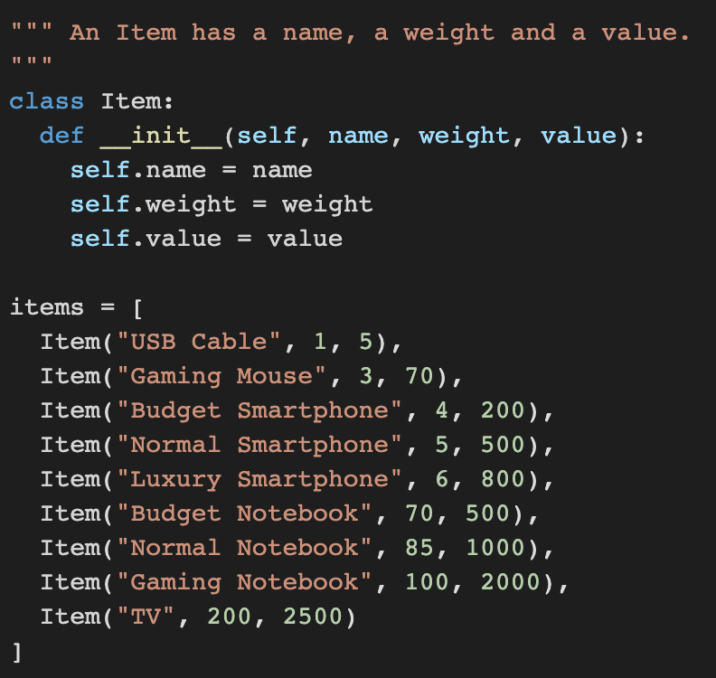
We define the Items for the knapsack by creating a Item class and adding items to the Items list :

The following is a recursive solution for the knapsack problem with an exponential time complexity $\mathcal{O}(2^n)$, which is unsuitable for large n = amount of items:

1.2 Greedy (subobtimal solution but fast)

A greedy algorithm makes locally optimal choices at each step of a problem-solving process in order to arrive at a global solution. The algorithm follows the principle of "making the best choice at the current moment without considering future consequences". It is simple and efficient and commonly used in optimization problems, with a time complexity of $\mathcal{O}(n)$ or $\mathcal{O}(n\log(n))$. However, greedy algorithms do not always guarantee optimal solutions. The following code shows a greedy solution for the knapsack problem which sorts items by their value-to-weight ratio with a time complexity of $\mathcal{O}(n\log(n))$:

1.3 Backtracking (optimal solution but not too fast)

Backtracking is a problem-solving technique that involves constructing a candidate solution incrementally and backtracks when a contradiction is reached, with the aim of finding a valid solution. Efficient backtracking algorithms rely on two key ingredients: look-ahead and pruning. Look-ahead involves ordering the search space such that the most relevant solutions are considered first, while pruning identifies sub-optimal paths early and discards them without explicitly checking. The recursion algorithm in 1.1 can be seen as an inefficient backtracking algorithm.
The following is a more efficient backtracking solution, which sorts items by their value-to-weight ratio and prunes, but still has a time complexity of $\mathcal{O}(2^n)$:

1.4 Dynamic Programming (optimal solution, fast, but uses extra memory)

Dynamic programming is a technique to reduce the time complexity of an algorithm by utilizing extra memory. It involves dividing a problem into sub-problems that can be optimized independently, with intermediate results stored to avoid duplicate computations. Knapsack problem can be solved using dynamic programming, and a value matrix V is stored where $V\left[ i \right]\left[ c \right]$ is the maximum value that can be achieved with capacity c using only the first i items. The time complexity of the dynamic programming approach is $\mathcal{O}(n \cdot \text{capacity})$, and its space complexity is also $\mathcal{O}(n \cdot \text{capacity})$. There are two approaches to dynamic programming: bottom-up and top-down. 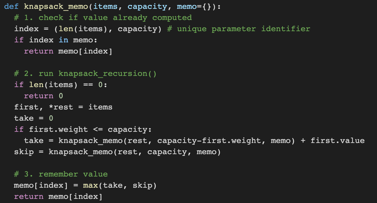Bottom-up dynamic programming algorithms begin computing the entries of the matrix starting with the simple cases, while top-down dynamic programming algorithms implement memoization to avoid duplicate computations by storing intermediate results.
The following shows a solution using bottom-up dynamic programming with time complexity of $\mathcal{O}(n \cdot \text{capacity})$:

The following uses top-down dynamic programming and memorization with time complexity of $\mathcal{O}(\min(2^n,n\cdot \text{capacity}))$:

1.5 Linear Programming (when having multiple contraints)

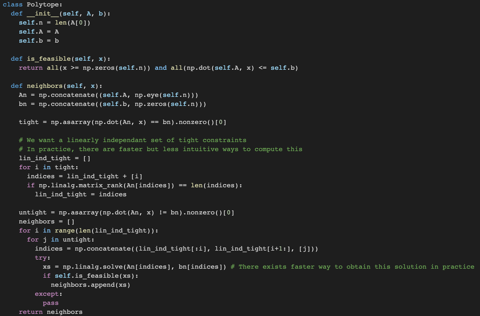
Linear programming is a method of optimizing a linear function subject to a set of linear constraints. It is a mathematical technique used to determine the best possible outcome from a given set of constraints. The set of feasible points of an LP corresponds to an n-dimensional convex polytope. The simplex algorithm is a popular method used to solve LPs, which starts from a node of the LP polytope and jumps to neighboring nodes having better objectives until the optimal solution is reached. However, the time complexity of the simplex algorithm can be exponential in the size of the input. Other LP algorithms, known as interior point methods, are provably faster.
The following shows the simplex algorithm alongside the polytope definition:

1.6 Linear Relaxation (turning ILP into LP problems)

Linear relaxation is a common technique used in optimization problems where we replace the integer constraints in an integer linear program (ILP) with relaxed constraints that allow for non-integer values. This results in a linear programming (LP) problem that can be solved using efficient algorithms such as the simplex method. However, the solution obtained from the LP relaxation may not be integer-valued and may need to be rounded to obtain a feasible solution for the original ILP.

While there is no guarantee that the solution obtained from the LP relaxation is optimal for the original ILP, there are certain classes of constraint matrices, such as totally unimodular matrices, for which the LP relaxation solution is indeed optimal for the original ILP. Additionally, linear relaxation can be used as a preprocessing step to obtain a good initial solution for other optimization algorithms.

1.7 Flows (For Solving Graphs with Nodes and Edges)

Flows are algorithmic concepts that are related to linear programming and linear relaxations. Graphs and flows are useful to model transportation networks of goods from source node s to target node t in a company. The formal definition of an s-t flow is a function $f: E → R_{\ge 0}$ such that

The maximum flow that can be established between a source and a target node in a network is the maximum flow problem. The integral flow theorem states that there exists a maximum flow such that every edge has an integral flow. The linear relaxation of the ILP formulation and the simplex algorithm can be used to solve a discrete maximum flow problem. Alternatively, there are more efficient algorithms known as augmenting paths algorithms. 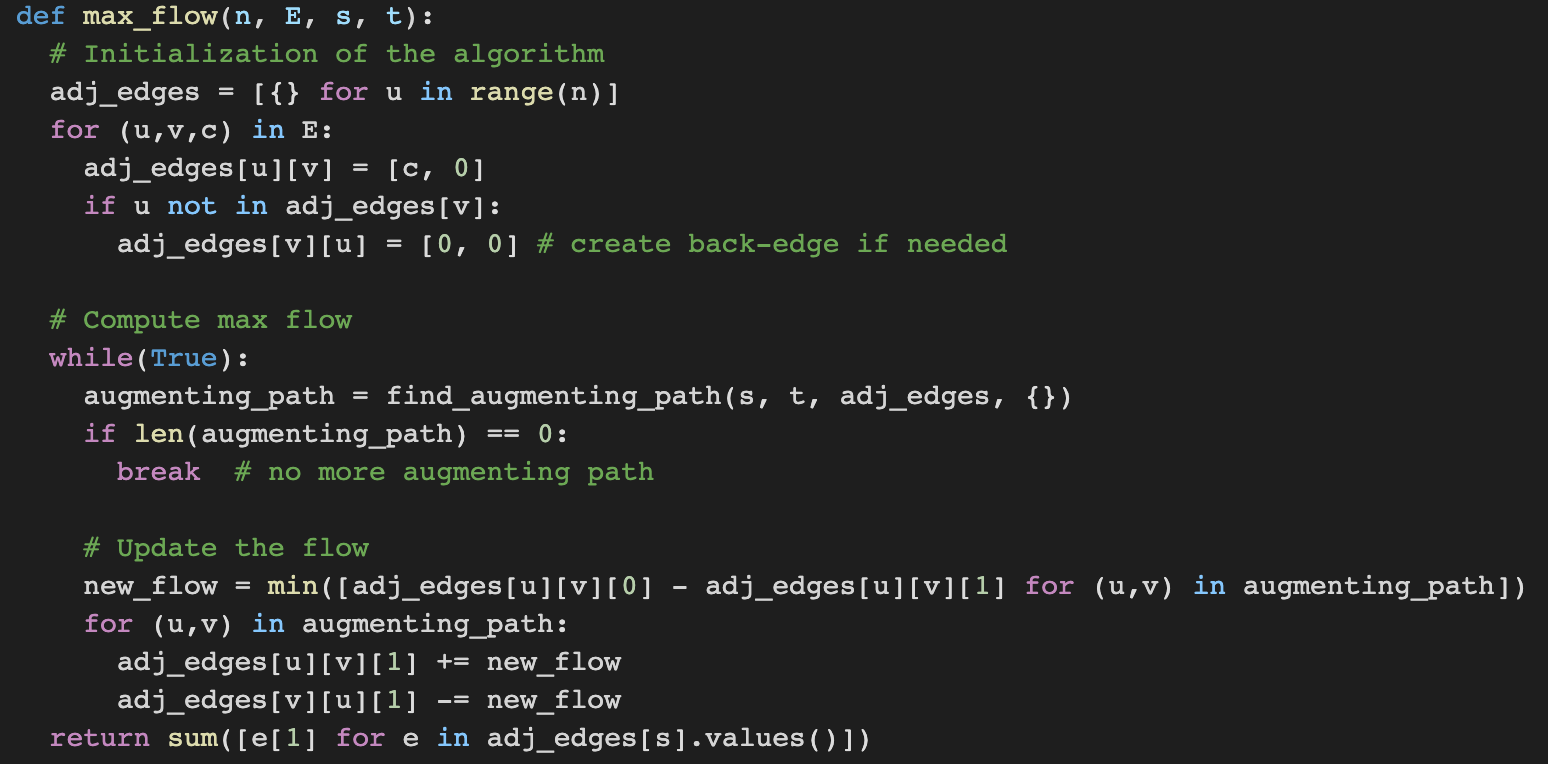The flow f is represented by one variable $x(u,v)$ for every directed edge $(u,v) \in E$ that indicates the value on that edge, and an augmenting path is a path from s to t such that the flow of each edge does not reach its capacity or flow can be pushed back.
The following shows the Ford Fulkerson algorithm to slove the flow problem:

2. Complexity

3. Cryptography

4. Databases

5. Machine Learning