Chapter 10 Response surface methods
10.1 Introduction
In the previous chapters, we were concerned with comparative experiments using categorical or qualitative factors, where each factor level is a discrete category and there is no specific order in the levels. We took a small detour into the analysis of ordered factors in Section 5.1.6. In this chapter, we consider designs to explore and quantify the effects of several quantitative factors on a response, where factor levels considered in an experiment are chosen from an infinite range of possible levels. Examples of such factors are concentrations, temperatures, and durations.
We are interested in two main questions: (i) to describe how changing the level of one or more factors affects the response and (ii) to determine factor levels that maximize (or minimize) the response. For addressing the first question, we consider designs that experimentally determine the response at specific points around a given factor setting and use a simple regression model to interpolate or extrapolate the expected response values at other points. For addressing the second question, we first explore how the response changes around a given setting, determine the factor combinations that likely yield the highest increase in the response, experimentally evaluate these combinations, and then start over by exploring around the new ‘best’ setting. This idea of sequential experimentation for optimizing a response was introduced in the 1940s (Hotelling 1941) and we discuss response surface methodologies (RSM) introduced by George Box and co-workers in the 1950s (Box and Wilson 1951,@Box1954) as a set of powerful and flexible techniques for implementing a sequential experimentation strategy. These techniques are commonly applied in biotechnology to find optimal conditions for a bioprocess to maximize yield, e.g., temperatures, pH, and flow rates in a bioreactor. Our example is more research-oriented and concerns optimizing the composition of a yeast growth medium, where we measure the number of cells after some time as the response, and consider the concentration (or amount) of five ingredients—glucose Glc, two nitrogen sources N1 and N2, and two vitamin sources Vit1 and Vit2—as our treatment factors.
10.2 The response surface model
The key new idea in this chapter is to consider the response as a smooth function, called the response surface, of the quantitative treatment factors. We generically call the treatment factor levels \(x_1,\dots,x_k\) for \(k\) factors, so that we have five such variables for our example, corresponding to the five concentrations of medium components. We again denote the response variable by \(y\), which is the increase in optical density in a defined time-frame in our example. The response surface \(\phi(\cdot)\) is then \[ y = \phi(x_{1},\dots,x_{k}) + \varepsilon\;, \] and relates the expected response to the experimental variables.
We assume that small changes in the amounts will yield small changes in the response, so the surface described by \(\phi(\cdot)\) is smooth enough that, given two points and their resulting response, we feel comfortable in interpolating intermediate responses. The shape of the response surface and its functional form \(\phi(\cdot)\) are of course unknown, and each measurement of a response is additionally subject to some variability \(\varepsilon\). The goal of a response surface design is to define \(n\) design points \((x_{1,j},\dots,x_{k,j})\), \(j=1\dots n\), and use a reasonably simple yet flexible regression function to approximate the true response surface from the resulting measurements \(y_j\), at least locally around a specified point. This approximation allows interpolation of the expected response for any combination of factor levels that is not too far outside the region that we explored experimentally.
Having found such approximation, we can determine the path of steepest ascent, the direction along which the response surface increases the fastest. For optimizing the response, we design a next experiment where we consider design points along this gradient (the gradient pursuit experiment). Having found a new set of conditions that gives higher expected yield than our starting condition, we iterate the two steps: locally explore the response surface around the new best treatment combination, approximate the surface and determine the gradient, and follow this gradient in a subsequent experiment. We follow this procedure until no further improvement of the measured response is observed, we found a treatment combination that yields a satisfactorily high response, or we run out of resources. This idea of a sequential experimental strategy is illustrated in Figure 10.1 for two treatment factors whose levels are on the horizontal and vertical axis, and a response surface shown via its contours.
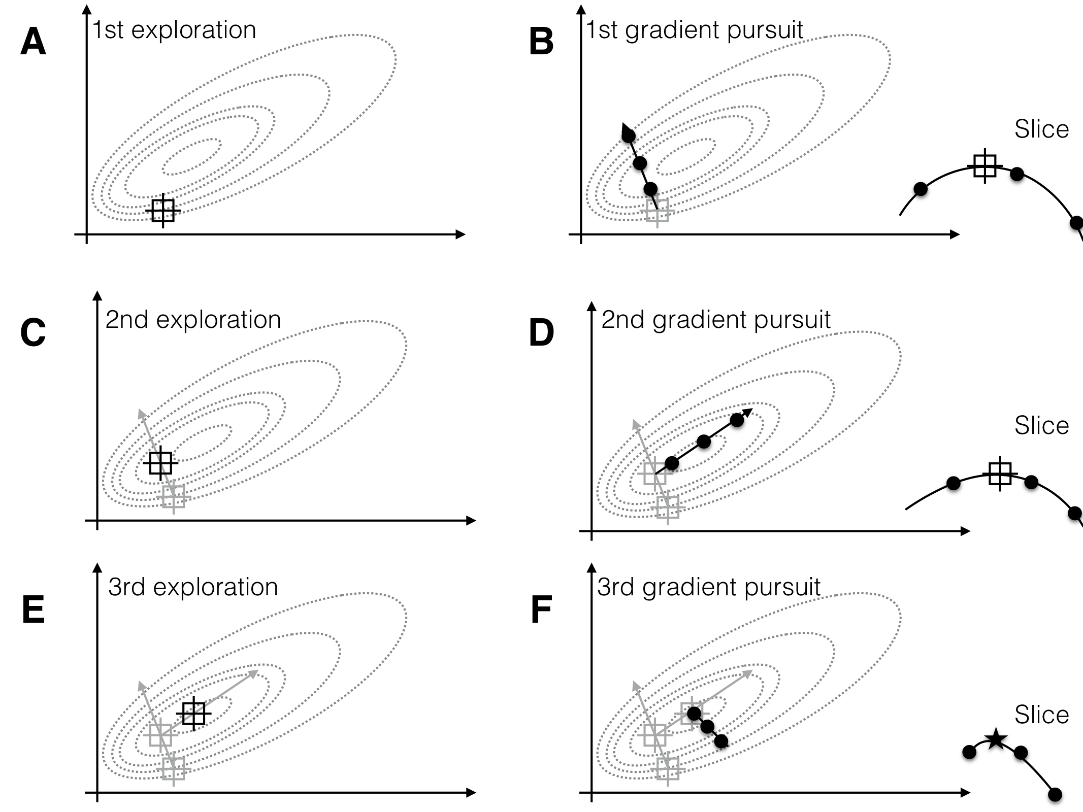
Figure 10.1: Sequential response surface experiments to determine optimum conditions. Three iterations of exploration (A,C,E) and gradient pursuit (B,D,F). Dotted lines: contours of response surface. Black lines and dots: region and points for exploring and gradient pursuit. Inlet curves in panels B,D,F show the slice along the gradient with measured points and resulting estimated maximum.
For implementing this strategy, we need to answer several questions: (i) what point do we start from?; (ii) how do we approximate the surface \(\phi(\cdot)\) locally?; (iii) how many and what design points \((x_{1,j},\dots,x_{k,j})\) do we choose to estimate this approximation?; and (iv) how do we determine the path of steepest ascent?
Optimizing treatment combinations usually means that we already have a reasonably reliable experimental system, so we use the current experimental condition as our initial point for the optimization. An important aspect here is the reproducibility of the results: if the system or the process under study does not give reproducible results at the starting point, there is little hope that the response surface methodologies will give better results.
The remaining four questions are very interdependent: we typically opt for simple (polynomial) functions to locally approximate the response surface. Our experimental design must then allow the estimation of all parameters of this function, the estimation of the residual variance, and ideally provide information to separate residual variation from lack of fit of the approximation. Determining a gradient is straightforward for polynomial interpolation function.
We discuss two options: the linear (first-order) interpolation and the quadratic (second-order) interpolation. A second-order polynomial accounts for curvature in the response surface, at least locally, and this interpolation always has a minimum or maximum. In contrast, a first-order polynomial is essentially a plane and continues increasing or decreasing indefinitely. An advantage is the reduced number of parameters and therefore experimental conditions required, and first-order polynomials are suitable for the first rounds of iteration, when we are likely far away from the actual optimum and only need a rough direction to follow. Second-order polynomials can then be used in subsequent iterations to provide a more accurate approximation and additional information about the response surface, but they require more complex designs.
10.3 The first-order model
We start our discussion by looking into the first-order model for locally approximating the response surface. Theory, calculations, and experimental designs are easier than for the second-order model, which helps us get acquainted with the general principles before moving to slightly more advanced ideas.
10.3.1 Model
The first-order model for \(k\) quantitative factors is \[ y = \phi(x_1,\dots,x_k) + \epsilon = \beta_0 + \beta_1 x_1 +\cdots+\beta_k x_k +\epsilon = \beta_0 + \sum_{i=1}^k \beta_{i} x_i + \varepsilon\;. \] Its parameters are estimated using simple linear regression with no interaction between factors. As in linear regression, the parameter \(\beta_i\) gives the amount by which the expected response \(y\) increases if we increase the \(i\)th factor from \(x_i\) to \(x_i+1\), while keeping all other factors at their current value. Because the model has no interaction terms between its factors, the increase in response affected by changing \(x_i\) is predicted to be independent of the values of all other factors. This is clearly an oversimplification in most applications. We assume the same constant error variance \(\text{Var}(\varepsilon)=\sigma^2\) everywhere; this is justified by the fact that we explore the response surface in the vicinity of a given starting point, so even if the variance is not constant over a larger range, it will usually be very similar at points not too far apart. For our example, the first-order model has one grand mean \(\beta_0\) and five parameters \(\beta_1,\dots,\beta_5\), one for each treatment factor.
10.3.2 Direction of steepest ascent
At any given point \((x_1,\dots,x_k)\), we determine the direction in which the response increases the fastest by calculating the gradient. For a first-order model, the gradient is \[ g(x_1,\dots,x_k) = \left(\frac{\partial}{\partial x_1} \phi(x_1,\dots,x_k), \dots, \frac{\partial}{\partial x_k} \phi(x_1,\dots,x_k)\right)^T = \left(\beta_1,\dots,\beta_k\right)^T\;. \] We estimate the gradient by plugging in the estimated parameters: \(\hat{g}(x_1,\dots,x_k)=\left(\hat{\beta}_1,\dots,\hat{\beta}_k\right)^T\). For first-order response surface models, the gradient is independent of the factor levels (the function \(g(\cdot)\) does not depend on any \(x_i\)), and the direction of steepest ascent is the same no matter where we start.
In the next iteration, we can then explore only this direction experimentally to find an experimental condition that yields higher expected response then our starting condition. In principle, the first-order model predicts ever-increasing response values along the gradient. In practice, the local approximation of the actual response surface by our first-order model is likely to fail once we venture far enough from the starting condition, and we will encounter decreasing responses and increasing discrepancies between the response predicted by the approximation and the response actually measured. The first round of exploration and gradient pursuit for a first-order model is illustrated in Figure 10.2.
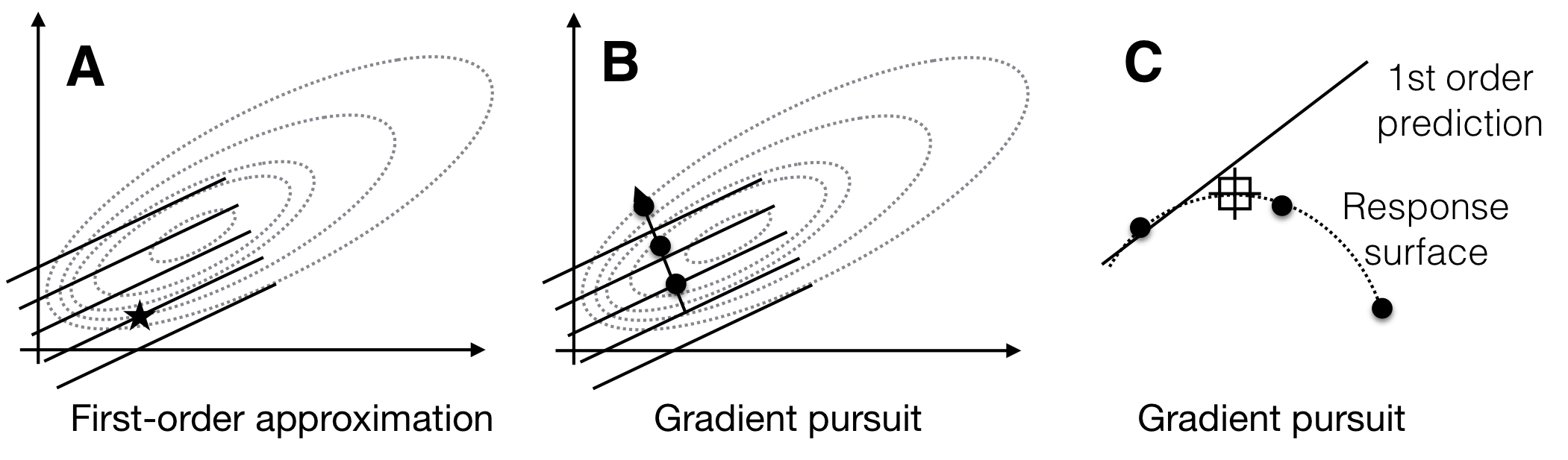
Figure 10.2: Sequential response surface experiment with first-order model. A: The first-order model (solid lines) build around a starting condition (star) approximates the true response surface (dotted lines) only locally. B: The gradient follows the increase of the plane and predicts indefinite increase in response. C: The first-order approximation (solid line) deteriorates from the true surface (dotted line) at larger distances from the starting condition, and the measured responses (points) start to decrease.
10.3.3 Experimental design
The first-order model with \(k\) factors has \(k+1\) parameters, and estimating these requires at least as many observations at different design points. Two options for an experimental design are shown in Figure 10.3 for a two-factor design. In each design, we consider three different levels for each factor: the level at the starting condition, called center, and one level lower and higher each. In the first design (Fig. 10.3A), we keep all factors at their starting condition level, and only change the level for one factor at a time. This yields two axial points for each factor, and the design resembles a coordinate system centered at the starting condition. The second design (Fig. 10.3B) is a full \(2^2\)-factorial where all factorial points are considered. This design would allow estimation of interactions between the factors and thus a more complex form of approximation. For our purposes, the first design would be adequate since our first-order model does not include interactions and therefore does not require measuring response values at different factor level combinations.
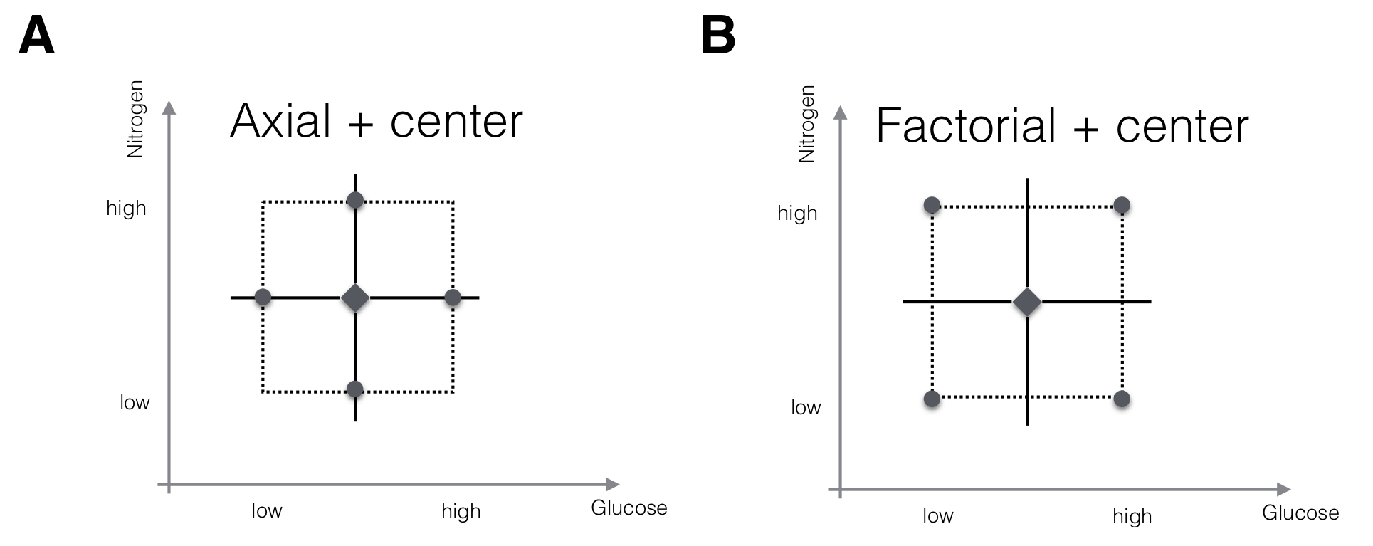
Figure 10.3: Two designs for fitting a first-order RSM with two factors. A: Center points and axial points that modify the level of one factor at a time only allow estimation of main effects, but not of interaction. B: Center points and factorial points would allow estimation of interactions but increase the experiment size.
In both designs, we additionally use several replicates at the starting condition as center points. This allows us to estimate the residual variance independently of any assumed model. Comparing this estimate with the observed discrepancies between any other point of the predicted response surface and its corresponding measured value allow to test more generally the goodness of fit of our model. In particular, we observe each factor at three levels, and we can use this additional information detect curvature not accounted for by the first-order model.
With \(k\) factors and \(m\) replicate measurements at the center point, the first design requires \(2k+m\) measurements. For the factorial design, \(2^k+m\) measurements are required, but fractional factorials often reduce the experiment size.
A problem of practical importance is then the choice for the low and high level of each factor. When chosen too close to the center point, the values for the response will be very similar and it is unlikely that we detect anything but large effects if the residual variance is not very small. When chosen too far apart, we might ‘brush over’ important features of the response surface and end up with a poor approximation. Only subject-matter knowledge can guide us in choosing these levels satisfactorily; for biochemical factors, one-half and double the starting concentration is often a reasonable first guess.16
10.3.4 Example: yeast medium optimization
For the yeast medium optimization, we consider a \(2^5\)-factorial augmented by six replicates of the center point. This design requires \(2^5+6=32+6=38\) runs, which we reduce to \(2^{5-1}+6=16+6=22\) runs using a half-replicate of the factorial. The design is given in Table 10.1, where low and high levels are encoded as \(\pm 1\) and the center level as 0 for each factor, irrespective of the actual amounts or concentrations. This encoding ensures that all parameters have the same interpretation as twice the expected difference in response between low and high level, irrespective of the numerical values of the concentrations used in the experiment. In addition, it centers the design at the origin of the coordinate system, with the center points having coordinate \((0,0,0,0,0)\). The last column shows the measured differences in optical density, with higher values indicating more cells in the corresponding well.
In R, response surface designs can be generated and analysed using the rsm package (Lenth 2009), which contains the utility function coded.data() that allows re-scaling the original treatment factor levels to the \(-1/0/+1\) scale. The following code is used for our example:
# Code factor levels in dataframe 'rsm1' to -1 / 0 /+1
# Original factors are Glc etc, coded are named xGlc etc.
rsm1 = coded.data(rsm1,
                  xGlc ~ (Glc-40) / 20,     # uncoded: 20/40/60
                  xN1 ~ (N1-100) / 50,      # uncoded: 50/100/150
                  xN2 ~ (N2-50) / 50,       # uncoded: 0/50/100
                  xVit1 ~ (Vit1-30) / 15,   # uncoded: 15/30/45
xVit2 ~ (Vit2-100) / 100) # uncoded: 0/100/200| xGlc | xN1 | xN2 | xVit1 | xVit2 | delta |
|---|---|---|---|---|---|
| Factorial points | |||||
| -1 | -1 | -1 | -1 | 1 | 1.74 |
| 1 | -1 | -1 | -1 | -1 | 0.13 |
| -1 | 1 | -1 | -1 | -1 | 1.48 |
| 1 | 1 | -1 | -1 | 1 | -0.01 |
| -1 | -1 | 1 | -1 | -1 | 120.21 |
| 1 | -1 | 1 | -1 | 1 | 140.31 |
| -1 | 1 | 1 | -1 | 1 | 181.00 |
| 1 | 1 | 1 | -1 | -1 | 39.97 |
| -1 | -1 | -1 | 1 | -1 | 5.80 |
| 1 | -1 | -1 | 1 | 1 | 1.44 |
| -1 | 1 | -1 | 1 | 1 | 1.45 |
| 1 | 1 | -1 | 1 | -1 | 0.64 |
| -1 | -1 | 1 | 1 | 1 | 106.37 |
| 1 | -1 | 1 | 1 | -1 | 90.94 |
| -1 | 1 | 1 | 1 | -1 | 129.06 |
| 1 | 1 | 1 | 1 | 1 | 131.55 |
| Center point replicates | |||||
| 0 | 0 | 0 | 0 | 0 | 81.00 |
| 0 | 0 | 0 | 0 | 0 | 84.08 |
| 0 | 0 | 0 | 0 | 0 | 77.79 |
| 0 | 0 | 0 | 0 | 0 | 82.45 |
| 0 | 0 | 0 | 0 | 0 | 82.33 |
| 0 | 0 | 0 | 0 | 0 | 79.06 |
Parameter estimation for the first-order model is straightforward using R’s linear regression function lm(). A very useful alternative is rsm() from the rsm package which augments R’s model specification formulae with several shortcuts, works directly with coded data, and provides more information specific to response surfaces in its output that we would need to calculate manually otherwise. The first-order model is specified using the shortcut FO() as r.fo = rsm(delta~FO(xGlc,xN1,xN2,xVit1,xVit2), data=rsm1).
The summary output of this model is found using summary(m) and is divided into three parts: first, the parameter estimates \(\hat{\beta}_0,\dots,\hat{\beta}_5\) shown in Table 10.2. With coded data, each parameter is the average difference between the low (resp. high) level of each factor and the starting level. We note that N2 has the largest impact and should be increased, that Vit2 should also be increased, that Glc should be decreased, while N1 and Vit1 seem to have only a comparatively small influence.
| Estimate | Std. Error | t value | Pr(>|t|) | |
|---|---|---|---|---|
| (Intercept) | 65.4 | 5.485 | 11.92 | 2.255e-09 |
| xGlc | -8.885 | 6.431 | -1.382 | 0.1861 |
| xN1 | 1.137 | 6.431 | 0.1768 | 0.8619 |
| xN2 | 57.92 | 6.431 | 9.006 | 1.155e-07 |
| xVit1 | -1.098 | 6.431 | -0.1708 | 0.8665 |
| xVit2 | 10.98 | 6.431 | 1.707 | 0.1072 |
Second, the summary output provides an ANOVA table shown in Table 10.3, which partitions the sums of squares for this model into three components: the major portion is explained by the first-order model, indicating that the five factors indeed affect the number of cells. The residuals with 16 degrees of freedom are further partitioned into the lack of fit and the pure error. The lack of fit is substantial, with a highly significant \(F\)-value, and the first-order approximation is clearly not an adequate description of the response surface. This is to be expected with such a simple approximation, but the resulting parameter estimates already give a clear indication for the next round of experimentation along the gradient. Recall that we are not interested in finding an adequate description of the surface at this point, our main goal is to find the direction of highest increase in the response values. For this, the first-order model should suffice for the moment. The pure error is based solely on the six replicates of the center points and consequently has five degrees of freedom. The residual variance is about 5.5 and very small compared to the other contributors. This means that (i) the starting point produces highly replicable results and (ii) small differences on the response surface are detectable (the residual standard deviation is about 2.4, and the difference between low and high glucose concentration, for example, is already \(2\cdot (-8.9)\approx 17.8\)).
| Df | Sum Sq | Mean Sq | F value | Pr(>F) | |
|---|---|---|---|---|---|
| FO(xGlc, xN1, xN2, xVit1, xVit2) | 5 | 56908 | 11382 | 17.2 | 6.192e-06 |
| Residuals | 16 | 10589 | 661.8 | ||
| Lack of fit | 11 | 10561 | 960.1 | 175.6 | 9.732e-06 |
| Pure error | 5 | 27.34 | 5.468 |
Third, the output provides the resulting gradient, as shown in Table ??, indicating the direction of steepest ascent in standardized (encoded) coordinates.
| xGlc | xN1 | xN2 | xVit1 | xVit2 |
|---|---|---|---|---|
| -0.149 | 0.01907 | 0.9712 | -0.01842 | 0.1841 |
10.4 The second-order model
The second-order model augments the first-order model by accounting for curvature in the response surface and by explicitly incorporating interactions between the treatment factors. Unless the response surface is highly irregular, a second-order model should provide an adequate local approximation around an optimum. The higher number of parameters and the higher-order terms in this model require larger and more complex experimental designs, but these are still very manageable even for moderate number of factors.
10.4.1 Model
The second-order model adds purely quadratic (PQ) terms \(x_i^2\) and two-way interaction (TWI) terms \(x_i\cdot x_j\) to the first-order model (FO), such that the regression model equation becomes \[ y = \phi(x_1,\dots,x_k)+ \epsilon = \beta_0 + \sum_{i=1}^k \beta_{i} x_i + \sum_{i=1}^k \beta_{ii} x_i^2 + \sum_{i<j}^k \beta_{ij} x_ix_j +\varepsilon\;, \] and we again assume a constant error variance \(\text{Var}(\epsilon)=\sigma^2\) for all points (and can again justify this because we are looking at a local approximation of the response surface). For example, the two-factor second-order response surface model is \[ y = \beta_0 + \beta_1 x_1+\beta_2 x_2 + \beta_{1,1}x_1^2 + \beta_{2,2}x_2^2 + \beta_{1,2} x_1x_2+\varepsilon\;. \]
The second-order model avoids the limitations of a linear surface by allowing curvature in all directions and interactions between factors while still requiring the estimation of only a reasonable number of parameters. Quadratic approximations are very common in statistics and applied mathematics, and perform satisfactorily for most problems, at least locally in the vicinity of a given starting point. Importantly, the model is still linear in the parameters, and parameter estimation can therefore be handled as a simple linear regression problem.
We can specify a second-order model using the rsm() function in package rsm and its convenient shortcut notation given in Table ??; note that SO() is the sum of FO(), PQ() and TWI(). Our example second-order model is specified as m=rsm(delta~SO(xGlc,xN1,xN2,xVit1,xVit2), data=rsm1).
Shortcuts for defining response surface models in rsm().
| Shortcut | Meaning | Example for two factors |
|---|---|---|
FO() |
First-order | \(\beta_0+\beta_1\, x_1+\beta_2\, x_2\) |
PQ() |
Pure quadratic | \(\beta_{1,1}\, x_1^2 + \beta_{2,2}\, x_2^2\) |
TWI() |
Two-way interactions | \(\beta_{1,2}\, x_1\,x_2\) |
SO() |
Second-order | \(\beta_0+\beta_1\, x_1+\beta_2\, x_2+\beta_{1,2}\, x_1\,x_2+\beta_{1,1}\, x_1^2 + \beta_{2,2}\, x_2^2\) |
10.4.2 Direction of steepest ascent
The gradient of the second-order model now depends on the position: for example, the first element of the gradient vector is \[ (g(x_1,\dots,x_k))_1 = \frac{\partial}{\partial x_1}\phi(x_1,\dots,x_k)=\beta_1 + 2\beta_{1,1} x_1 + \beta_{1,2} x_2 + \cdots +\beta_{1,k} x_k\;, \] and we typically compute the gradient starting at the center point. That means that the direction of steepest ascent changes as we follow this ascent, and the steepest path along the response surface can now be curved (as compared to the straight line of the first-order model). This path is often called the canonical path.
With a second-order model, we can also investigate the curvature of the response surface, at least locally. For this, we can use a canonical analysis, which first computes a new coordinate system, such that the quadratic surface’s main axes are parallel to the coordinate system, and the origin is at a specific point of interest, often a supposed maximum of the response. From the estimated surface equation, we can then determine how the approximation surface looks like; it could be a ‘hill’ with a clearly defined maximum; a ridge in which a combination of two or more factors can be varied in a constant proportion with only little change to the resulting response; or a saddle-point, in which certain directions increase the response, other decrease the response, and there is a stationary point in between. We will not discuss canonical analysis here, however, and refer to the texts by Box, Hunter, and Hunter (Box, Hunter, and Hunter 2005) and of Cox and Cochran (Cochran and Cox 1957), which both provide excellent discussions of response surface methods.
10.4.3 Experimental design
For a second-order model, we need at least three points on each axis to estimate its parameters and we need sufficient combinations of factor levels to estimate the interactions. An elegant way to achieve this is a center composite design (CCD). It uses center points with replication to provide a model-independent estimate of the residual variance, axial points, and a (fractional) factorial design to generate three points for each factor along a line parallel to its axis plus the factorial points for estimating interactions. This is a combination of the two designs we discussed for a first-order model and Figure 10.4 illustrates the CCD and its components for a design with two factors.
With \(m\) replicates of the center points, a central composite design for \(k\) factors requires \(2^k\) factorial points, \(2\cdot k\) axial points, and \(m\) center points. For large enough \(k\), the number of factorial points can be substantially reduced when considering fractional factorial designs. Since we estimate main effects and two-way interactions, a resolution of V is required for unconfounded estimation of parameters. For our example with \(k=5\) factors, the full CCD with six replicates of the center points requires measuring the response for \(32+10+6=48\) settings. The \(2_{\text{V}}^{5-1}\) fractional factorial reduces this number to \(16+10+6=32\) and provides a very economic design.
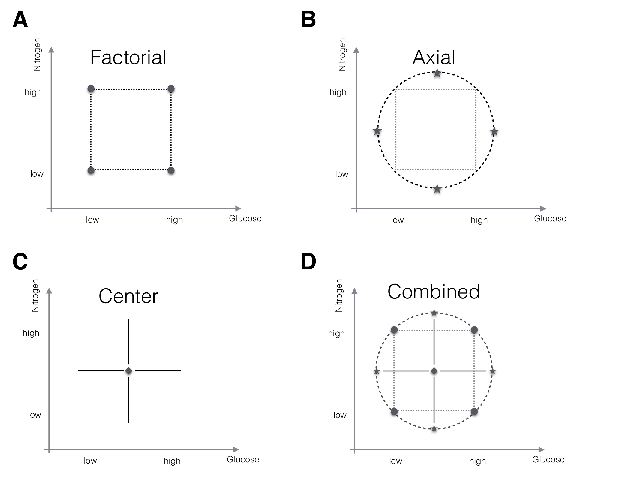
Figure 10.4: The components of a center composite design for two factors. A: (Fractional) factorial points for interactions. B: Axial points for quadratic effects. C: Center points for variance estimation. D: The full CCD design.
10.4.3.1 Choosing axial point levels
In the CCD, we combine axial points and factorial points, and so the question arises how to choose the two levels for each pair of axial points? There are two reasonable alternatives: First, use the same low/high levels as for the factorial design. The axial points then lie on the corresponding facet of the factorial hyper-cube and no new factor levels are introduced. For our example, this is a considerable advantage since it simplifies the different concentrations and associated buffers that need to be prepared for generating the different design points. The disadvantage is that the axial points are closer to the center points than are the factorial points and estimates of parameters then have different standard errors, leading to different variances of the model’s predictions depending on the direction.
Second, we can choose the axial points at the same distance from the center point as the factorial points. Then, the axial and factorial points lie on the same sphere centered at the center points, yielding a rotationally symmetric design as in Figure 10.4B. Since the factorial points have distance \(\sqrt{k}\) from the center, we set the low and high levels of the axial points as \(\pm \sqrt{k}\), and each factor is considered at the five levels \(-\sqrt{k},-1,0,+1,+\sqrt{k}\) in this design.
The idea of a center composite design is further illustrated for three factors in Figure 10.5. The top row shows the factorial (A), center, and axial points (B). Choosing the axial and factorial points to lie on the same sphere around the center yields a rotationally invariant design (C). Choosing the axial points to have the same factor levels already introduced by the center and factorial points yields a design with axial points on the facets of the factorial cube (D).
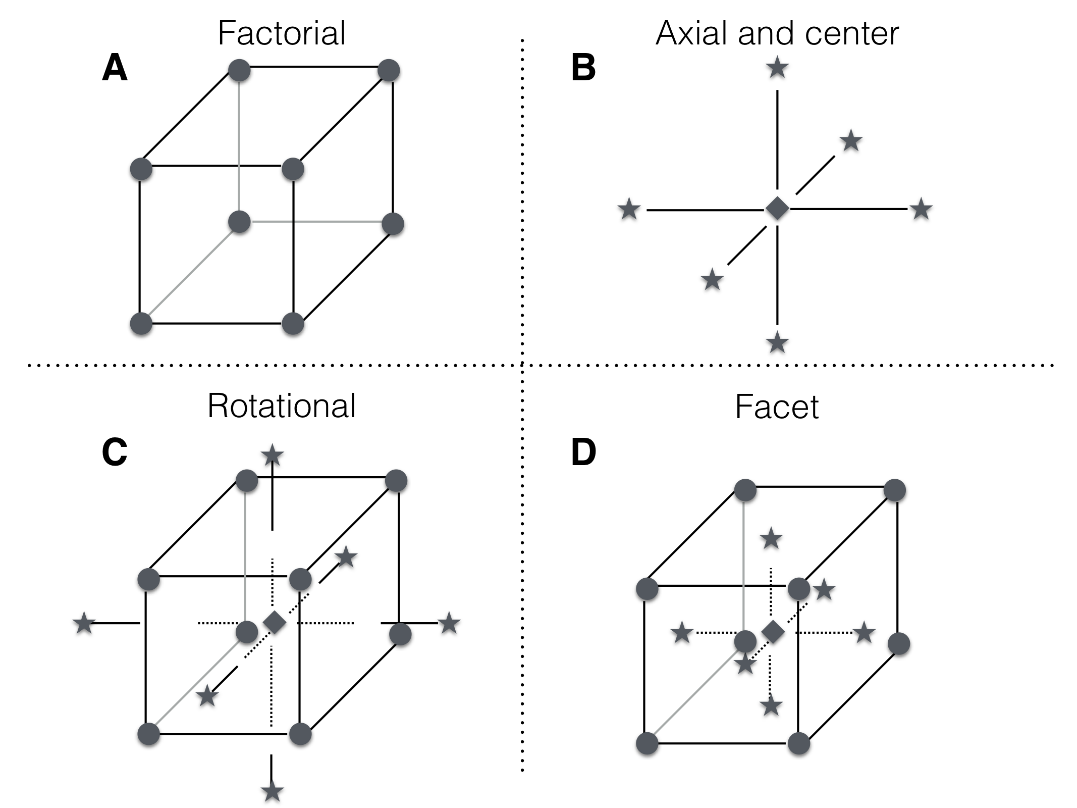
Figure 10.5: A center composite design for three factors. A: design points for \(2^3\) full factorial. B: center point location and axial points chosen along axis parallel to coordinate axis and through center point. C: combined design points yield center composite design, here with axis points chosen for rotatability and thus outside the cube. D: combined design points with axial points chosen on facets introduce no new factor levels.
10.4.3.2 Blocking a central composite design
An attractive feature of the central composite design is the fact that the sets of factorial and axial points are orthogonal to each other. This allows a very simple blocking strategy, where we use one block for the factorial points and some of the replicates of the center point, and another block for the axial points and the remaining replicates of the center point. We could then conduct the CCD of our example in two experiments, one with \(16+3=19\) measurements, and the other with \(10+3=13\) measurements, without jeopardizing the proper estimation of parameters. The block size for the factorial part can be further reduced using the techniques for blocking factorials from Section 9.8.
In practice, this property provides considerable flexibility when conducting such an experiment. For example, we might first measure the axial and center points and estimate a first-order model from these data and determine the gradient. With replicated center points, we are also able to determine the lack of fit of this model and gain insight into the curvature of the response surface. We might then decide to immediately continue with the gradient pursuit based on the first-order model if curvature is small, or to conduct a second experiment with factorial and center points to estimate the full second-order model. Alternatively, we might start with the factorial points to determine a factorial model with main effects and two-way interactions. Again, we can continue with these data alone, or augment the design with axial points to estimate the second-order model. Finally, if a CCD with fractional replication of the factorial points provides insufficient precision of the parameter estimates, we can augment the data with another fraction of the factorial design to disentangle confounded factors and to provide higher replication for estimating the model parameters.
A minor concern when blocking a central composite design is the number of center points per block to provide adequate estimation of the residual variance, and we might want to increase the total number of center points to ensure sufficient replication in each block. After accounting for block effects, we are then able to combine the data and produce a more precise estimate once all parts of the experiment have been implemented.
10.4.4 Sequential experiments
Given a highly symmetric and balanced design such as the CCD, estimating the parameters of a response surface is fairly straightforward. Once the parameters of the second-order model are found, we can use the model to determine the predicted maximum of the surface to find the optimal medium conditions. At least in the beginning of the experiment, our local approximation likely yields an optimum that is far outside the factor levels for which our experiment provides information. The predicted optimum is then rarely an optimum of the true response surface and is more likely an artifact of poor approximation of the true surface by our second-order model far outside the region for which data are available.
Our approach is therefore a sequential one: since the model is only a local approximation, we typically do not pursuit the optimum directly if it is too far away from the starting condition. Rather, we use the model to calculate the path of steepest ascent, which determines the fastest increase in response. For a second-order model, this path might not be a straight line but is easily calculable using software such as the rsm package. In a subsequent experiment, we follow this path and measure the response at different distances from our center point. A comparison of predicted and measured responses provides information about the range of factor levels for which the second-order model provides accurate predictions and is thus a good approximation of the true surface. We determine the point on the path with largest response and use this condition as our new center point to further explore the response surface around this new best experimental condition.
The procedure of exploring the surface by estimating a local second-order model around a center point, following the path of steepest ascent, and determining the new center points along the gradient is repeated until we either reach a maximum or we stop because we are satisfied with the improvement and do not want to invest more resources in further exploration.
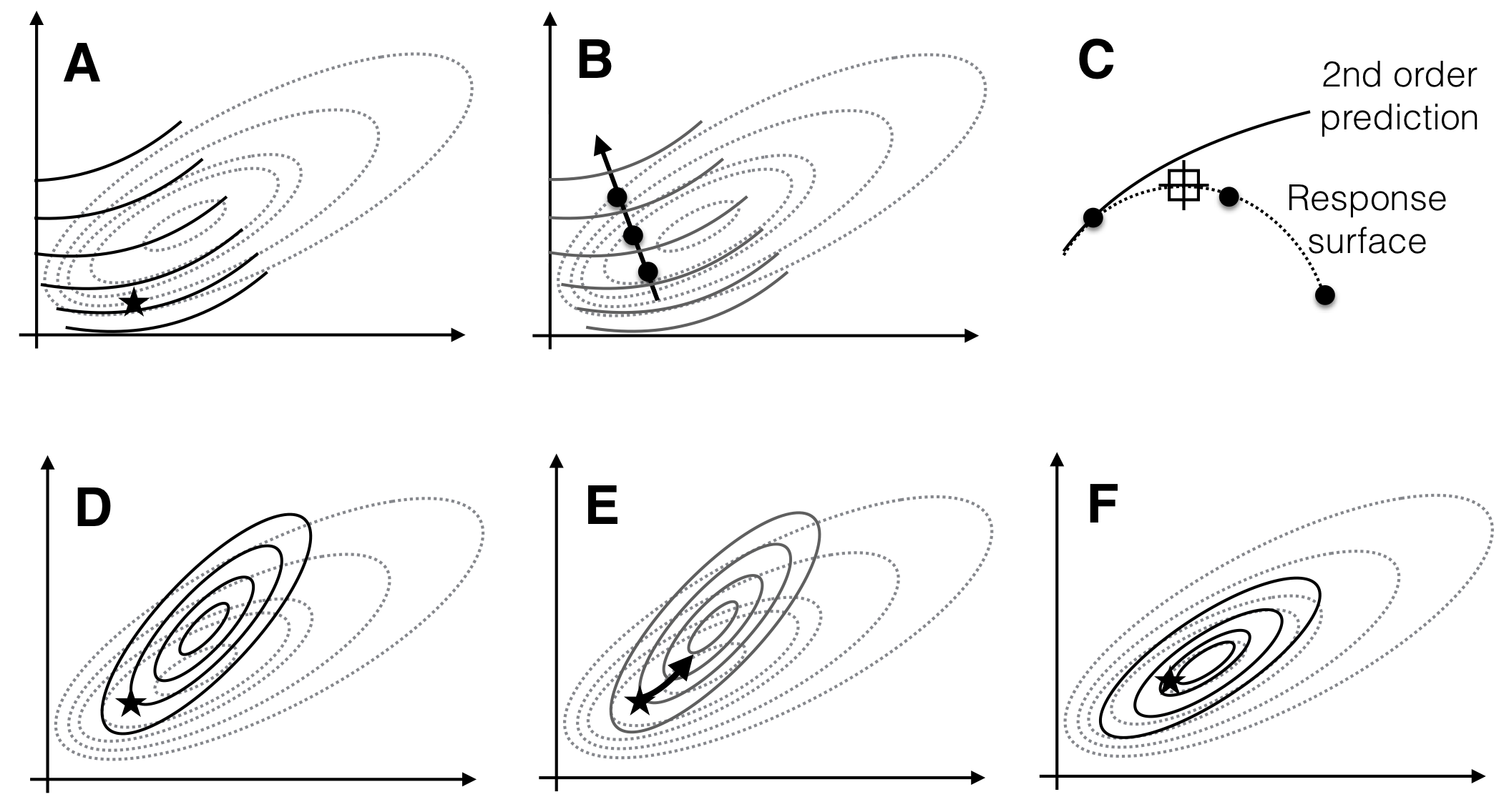
Figure 10.6: Sequential experimentation for optimization of conditions using second-order approximations. A: first approximation (solid lines) of true response surface (dotted lines) around a starting point (star) only describes the local increase towards the top-left. B: pursuing the path of steepest ascent yields a new best condition, but prediction and measurements diverge further out from the starting point. C: a slice along the path of steepest ascent highlights the divergence and the new best condition. D: second approximation around new best condition. E: path of steepest ascent based on second approximation. F: third approximation correctly identifies the optimum and captures the properties of the response surface around this optimum.
The overall sequential procedure is illustrated in Figure 10.6: the initial second-order approximation (solid lines) of the response surface (dotted lines) is only valid locally (A) and predicts an optimum far from the actual optimum, but pursuit of the steepest ascent increases the response values and moves us close to the optimum (B). Due to the local character of the approximation, predictions and measurements start to diverge further away from the starting point (C). The exploration around the new best condition predicts an optimum close to the true optimum (D) and following the steepest ascent (E) and a third exploration (F) achieve the desired optimization. The second-order model now has an optimum very close to the true optimum and correctly approximates the factor influences and their interactions.
10.5 Example: yeast growth medium optimization
We close the chapter with a more detailed discussion of a real-life example (Roberts, Kaltenbach, and Rudolf 2020). The goal is to find a growth medium composition for and other yeasts that yields a maximal number of cells at the onset of the diauxic shift. This medium, called high cell density (HCD) medium, is useful for biotechnology and for other applications such as transformation protocols that rely on high number of copied DNA, for example, and found a first application in miniaturization of a proteomics assay (???).
We consider glucose (Glc), monosodium glutamate (nitrogen source N1), a fixed composition of amino acids (nitrogen source N2), and two mixtures of trace elements and vitamins (Vit1 and Vit2) as the five ingredients whose composition we would alter. The response is the increase in optical density recorded by a reader on a 48-well plate, from onset of growth to the diauxic shift. Higher increase should indicate higher cell density.
Overall, we used two iterations of the sequential RSM, with a second-order approximation of the response surface followed by a pursuit of the steepest path. We discuss each of these four experiments in more detail.
10.5.1 First response surface exploration
Our choice for designing the response surface experiments required some alterations of the textbook procedure. There are two factors that largely influence the required effort and the likelihood of experimental errors: first, each experiment can be executed on a 48-well plate. Thus, any experiment size between 1 and 48 is roughly equivalent in terms of effort, because once an experiment is started, pipetting 48 wells does not take long. In addition, the ingredients are cheap, so cost was not a real issue here. In practical terms, that means that there is no point in starting with a first-order design and then augment it when necessary, because this strategy is more time-consuming than using a second-order model directly. This led to our decision to start from a standard yeast medium and use a \(2^{5-1}\) fractional factorial design together with 10 axial points (26 design points without center points) as our first experimental design.
Second, it is very convenient to use the same combinations of amounts for the five ingredients also for the axial points, so each component would only be required in three instead of five concentrations. This choice sacrifices the rotational symmetry of the design and leads to different standard errors since axial points are now closer to the center points than the factorial points. We considered this a small price to pay because pipetting is now easier and errors less likely.
We decided to use six center points to augment the five error degrees of freedom (26 observations in the design for 21 parameters in the second-order model). These allow separating lack of fit from residual variance and looking at the six resulting growth curves would also allow us to gauge the reproducibility of the original growth conditions and the bench protocol.
In this design, 16 wells of the 48-well plate remain unused. Since ingredients are cheap and pipetting twice is not much effort, we decided to replicate the fractional factorial part of the CCD in the remaining 16 wells, using a biological replicate (i.e., new yeast culture, independent pipetting of the medium compositions). This would give us replicates for these 16 points that we could use for checking the variability of the data and would also provide ‘backup’ in case some of the original 16 factorial points failed for whatever reason. We found excellent agreement between the two replicates, providing confidence that the experiment worked satisfactorily and we could move to the next phase. A statistically more satisfying option would have been to use the remaining 16 design points to complete the \(2^{5-1}\) fractional factorial to a full \(2^5\)-factorial. This would have required more complex pipetting, however, and we would also not have a direct replicate of each point to test biological variability.
The resulting increases in optical density (OD) are shown in Figure 10.7. The six values for the center points show excellent agreement, indicating high reproducibility of the experiment. Moreover, the average increase in OD for the starting condition is 81.1, and we already identified a condition with a value of 181, corresponding to a 2.2-fold increase.
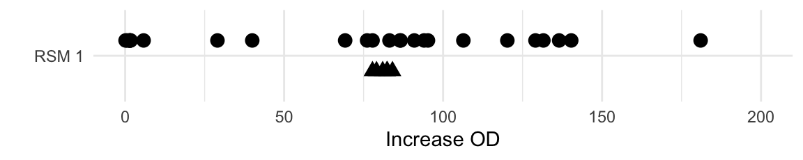
Figure 10.7: measured increase in OD for first exploration experiment. Triangles indicate center points and points are jitter on y-axis for better readability.
We next estimated the second-order approximation based on these observations and standardized values for the factor levels (\(-1/0/+1\)). The resulting parameter estimates showed several highly significant and large main effects and two-way interactions while the quadratic terms remained non-significant. This indicates that optimization cannot be done iteratively one factor at a time, but that several factors need to be changed simultaneously. The non-significant quadratic terms indicate that either the surface is sufficiently plane around the starting point, or that we chose factor levels too close together or too far apart to detect curvature. The ANOVA table for this model (Table 10.4), however, indicates that quadratic terms and two-way interactions as a whole cannot be neglected, but that the first-order part of the model is by far the most important:
| Df | Sum Sq | Mean Sq | F value | Pr(>F) | |
|---|---|---|---|---|---|
| FO(xGlc, xN1, xN2, xVit1, xVit2) | 5 | 62411 | 12482 | 139.7 | 1.441e-09 |
| TWI(xGlc, xN1, xN2, xVit1, xVit2) | 10 | 8523 | 852.3 | 9.538 | 0.0004329 |
| PQ(xGlc, xN1, xN2, xVit1, xVit2) | 5 | 4145 | 829.1 | 9.278 | 0.001144 |
| Residuals | 11 | 983 | 89.36 | ||
| Lack of fit | 6 | 955.6 | 159.3 | 29.13 | 0.0009759 |
| Pure error | 5 | 27.34 | 5.468 |
The table also suggests considerable lack of fit, but we expect this at the beginning of the optimization. This becomes very obvious when looking at the predicted stationary point of the approximated surface (Table ??), which contains negative concentrations and is far outside the region we explored in the first experiment (note that the units are given in standardized coordinates, so a value of 10 means ten times farther from the center point than our axial points).
| xGlc | xN1 | xN2 | xVit1 | xVit2 |
|---|---|---|---|---|
| -13.67 | 30.63 | 24.38 | 30.45 | 10.1 |
Further analysis also revealed this point to be a saddle point, which is neither a maximum nor a minimum.
10.5.2 First path of steepest ascent
Based on this second-order model, we calculate the path of steepest ascent for the second experiment. This is conveniently done using the steepest() function provided by rsm. This yields the path shown in Table 10.5.
| dist | Glc | N1 | N2 | Vit1 | Vit2 | yhat | Measured |
|---|---|---|---|---|---|---|---|
| 0.0 | 40.0 | 100.0 | 50.0 | 30.0 | 100.0 | 85.3 | 78.3 |
| 0.5 | 38.1 | 101.8 | 73.8 | 29.5 | 111.5 | 114.2 | 104.2 |
| 1.0 | 35.7 | 105.1 | 96.0 | 28.2 | 128.9 | 142.7 | 141.5 |
| 1.5 | 32.9 | 109.2 | 116.5 | 26.0 | 150.2 | 171.4 | 156.9 |
| 2.0 | 30.0 | 113.8 | 135.4 | 23.1 | 173.7 | 201.0 | 192.8 |
| 2.5 | 27.0 | 118.3 | 153.0 | 19.6 | 198.5 | 231.9 | 238.4 |
| 3.0 | 24.1 | 122.8 | 169.4 | 15.6 | 224.0 | 264.3 | 210.5 |
| 3.5 | 21.2 | 126.8 | 184.9 | 11.3 | 249.7 | 298.6 | 186.5 |
| 4.0 | 18.3 | 130.7 | 199.7 | 6.7 | 275.4 | 334.7 | 144.2 |
| 4.5 | 15.5 | 134.3 | 213.8 | 1.9 | 301.1 | 372.9 | 14.1 |
The first column shows the distance from the center point in standardized coordinates, so this path moves up to 4.5 times further than our axial points. The next columns show the resulting levels for our five treatment factors in standardized coordinates. The column yhat provides the predicted increase in OD based on the second-order approximation.
We experimentally followed this path and took measurements at the indicated medium compositions. This resulted in the measurements given in column Measured. We observe a fairly good agreement between prediction and measurement up to about distance 2.5 to 3.0. Thereafter, the predictions keep increasing while measured values drop sharply to almost zero. This is an example of exactly the situation depicted in Figure 10.6C, where the approximation breaks down further from the center point. This is clearly visible when graphing the prediction and measurements, as shown in Figure 10.8. Nevertheless, the experimental results show that along the path, an increase by about 3-fold compared to the starting condition can be achieved.
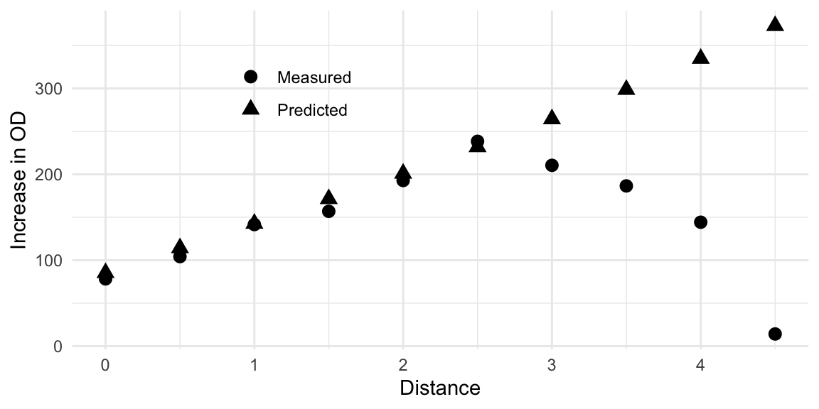
Figure 10.8: Comparison of observed growth values and predicted values along the path of steepest ascent. Model predictions deteriorate at a distance of about \(2.5-3.0\).
10.5.3 Second response surface exploration
Pursuing the gradient, we found a new experimental condition at about distance 2,5 from our starting condition that showed a 3-fold increase in growth. In the next iteration, we explored the response surface locally using a new second-order model centered at the current bats condition. We proceeded just as for the first RSM estimation, with a \(2^{5-1}\) design combined with axial points and six center point replicates.
The 32 observations from this experiment are shown in Figure 10.9 (top row) and look promising: several conditions showed further improvement of growth, although the fold-change in growth is considerably smaller than before. The maximal increase from the center point to any condition is about 1.5-fold. This is expected when we assume that we approach the optimum condition. The bottom row repeats the results from the first experiment.
Figure 10.9: Distribution of measured values for first (bottom) and second (top) exploration experiment with 32 conditions each. Triangular points are replicates of the corresponding center point condition.
The data also demonstrate the importance of replication of the center point and of having a reference condition in each experiment: in the second exploration, the center points showed much wider spread than in the first condition. This might be an indication of more difficult pipetting, especially considering that the center of the first exploration was a standard medium. An alternative explanation is that we approach the optimum of the response surface and experience more severe curvature. Slight deviations from the specified conditions might then have larger influence on the measured response, and increase measurement variation.
The new center conditions show consistently higher growth values than any condition of the first exploration. This is a good indication that the predicted increase from our gradient pursuit is indeed happening in reality. We also find several new conditions that yield even higher growth values, although their number is getting smaller compared to the number of conditions with lower growth.
Importantly, we do not have to compare the observed values between the two experiments directly: we can always retreat to comparing fold-changes in each experiment compared to its center point condition. Thus, if a value of 200 a.u. in the first experiment has a different meaning than 200 a.u. in the second experiment due to, e.g., changes in the calibration of the reader, this does not invalidate the optimization of the medium composition. Here, the values measured at the second center point conditions are around 230, which agrees perfectly with the predicted value from the gradient pursuit experiment, so we have confidence that the scales of the two experiments are directly comparable.
The estimated parameter for a second-order model now present a much cleaner picture: we find only main effects large and significant, and the interaction of glucose with the second nitrogen source (amino acids); all other two-way interactions and the quadratic terms are small. The ANOVA table (Tab. 10.6) still indicates some contributions of interactions and purely quadratic terms, but the lack of fit is now negligible. In essence, we are now dealing with a first-order model with one substantial interaction.
| Df | Sum Sq | Mean Sq | F value | Pr(>F) | |
|---|---|---|---|---|---|
| FO(xGlc, xN1, xN2, xVit1, xVit2) | 5 | 89756 | 17951 | 24.43 | 1.308e-05 |
| TWI(xGlc, xN1, xN2, xVit1, xVit2) | 10 | 33677 | 3368 | 4.582 | 0.009646 |
| PQ(xGlc, xN1, xN2, xVit1, xVit2) | 5 | 28321 | 5664 | 7.707 | 0.002453 |
| Residuals | 11 | 8084 | 734.9 | ||
| Lack of fit | 6 | 5978 | 996.3 | 2.365 | 0.1816 |
| Pure error | 5 | 2106 | 421.2 |
The model is still a very local approximation, as is evident from the stationary point, which again is far outside the region explored in this experiment and has several negative concentrations, as seen in Table ??.
| xGlc | xN1 | xN2 | xVit1 | xVit2 |
|---|---|---|---|---|
| 1.016 | -6.945 | 1.246 | -11.76 | -2.544 |
10.5.4 Second path of steepest ascent
Based on this second model, we again calculate the path of steepest ascent and follow it experimentally. The predictions and observed values are shown in Figure 10.10 and show excellent agreement between prediction and observation, even though the observed values are consistently higher than the predicted value. A plausible reason for this, especially since the shift also occurs at the starting condition, is a gap of several months between the second exploration experiment and the gradient pursuit experiment. This likely lead to new calibration of the fluorescence reader and several changes in the experimental apparatus, such that the ‘a.u.’ scale is now different from the previous experiments, apparently by shifting all values upwards by a fixed amount.
This systematic shift is not a problem in practice, since we are interested in fold changes, and the distance-zero condition along the gradient is identical to the previous center point. Thus, the ratio of any measured value to the value at distance zero provides a valid estimate of the increase in growth also compared to the previous center point condition of the second exploration experiment. Along the gradient, the growth is monotonically increasing, producing more and more cells; at the last condition, we achieved a further 2.2 fold increase compared to our previous optimum.
Figure 10.10: Comparison of observed growth values and predicted values along the gradient of steepest ascent.
Although our model predicts that further increase in growth is possible along the gradient, we stopped the experiment at this point: the wells of the 48-well plate were now crowded with cells. Moreover, we were not able to test the distance-5 medium composition, because several components were now so highly concentrated that salts started to fall out from the solution.
10.5.5 Further discussion
Overall, we achieved a 3-fold increase in the first iteration of RSM/gradient, followed by another increase of 2.2-fold in the second iteration, yielding an overall increase in growth of 6.8-fold. Given that previous manual optimization resulted in a less than 3-fold increase overall, this is a remarkable testament to the power of good experimental design and systematic evaluation and optimization of the medium composition.
The actual experiment used two replicates for the first RSM iteration. We also used the free wells of the 48-well plate in the second iteration to simultaneously determine the growth in several other growth media. The resulting comparisons are shown in Figure 10.11. The vertical axis shows the iterations of the experiment and the horizontal axis the increase in OD for each tested condition. Round points indicate trial conditions of the experimental design for RSM exploration or gradient pursuit, with grey shading denoting two independent replicates. During the second iteration, additional standard media (YPD and SD) were also measured in the same experiment to provide a direct control and comparison of the new HCD medium against established alternatives. Additionally, the second gradient pursuit experiment also repeated some of the previous exploration points for direct comparison.
A shift on the response variable is clearly seen for all conditions, and emphasizes the need for internal controls in each iteration. Nevertheless, the response increased by more than 6.5-fold from the initial medium composition to the best medium composition found along the second path of steepest ascent.
Figure 10.11: Summary of data acquired during four experiments in sequential response surface optimization. Additional conditions were tested during second exploration and gradient pursuit (point shape), and two replicates were measured for both gradients (point shading). Initial starting medium is shown as black point.
In the original experiment, we also noted that while increase in OD was excellent, the growth rate was much reduced compared to the starting medium composition. We addressed this problem by changing our optimality criterion from the simple increase in OD to the increase penalized by duration. Using the data from the second response surface approximation, we then calculated a new path of steepest ascent based on this modified criterion and arrived at the final medium described (Roberts, Kaltenbach, and Rudolf 2020) that provides both high density of cells and growth rates comparable to the initial medium; we refer the reader to the publication for details.
Abelson, Robert P., and Deborah A. Prentice. 1997. “Contrast tests of interaction hypothesis.” Psychological Methods 2 (4): 315–28. https://doi.org/10.1037/1082-989X.2.4.315.
Abelson, R P. 1995. Statistics as principled argument. Lawrence Erlbaum Associates Inc.
Bailar III, J. C. 1981. “Bailar’s laws of data analysis.” Clinical Pharmacology & Therapeutics 20 (1): 113–19.
Belle, Gerald van. 2008. Statistical Rules of Thumb: Second Edition. https://doi.org/10.1002/9780470377963.
Belle, Gerald van, and Donald C Martin. 1993. “Sample size as a function of coefficient of variation and ratio.” American Statistician 47 (3): 165–67.
Box, G E P. 1954. “The Exploration and Exploitation of Response Surfaces: Some General Considerations and Examples.” Biometrics 10 (1): 16. https://doi.org/10.2307/3001663.
Box, G. E. P., S. J. Hunter, and W. G. Hunter. 2005. Statistics for Experimenters. Wiley, New York.
Box, G E P, and K B Wilson. 1951. “On the Experimental Attainment of Optimum Conditions.” Journal of the Royal Statistical Society Series B (Methodological) 13 (1): 1–45. http://www.jstor.org/stable/2983966.
Buzas, Jeffrey S, Carrie G Wager, and David M Lansky. 2011. “Split-Plot Designs for Robotic Serial Dilution Assays.” Biometrics 67 (4): 1189–96. https://www.jstor.org/stable/41434424.
Cochran, W. G., and G. M. Cox. 1957. Experimental Designs. John Wiley & Sons, Inc.
Cohen, J. 1988. Statistical Power Analysis for the Behavioral Sciences. 2nd ed. Lawrence Erlbaum Associates, Hillsdale.
Cohen, J. 1992. “A Power Primer.” Psychological Bulletin 112 (1): 155–59.
Cox, D R. 1958. Planning of Experiments. Wiley-Blackwell.
Coxon, Carmen H., Colin Longstaff, and Chris Burns. 2019. “Applying the science of measurement to biology: Why bother?” PLOS Biology 17 (6): e3000338. https://doi.org/10.1371/journal.pbio.3000338.
Davies, O. L. 1954. “The Design and Analysis of Industrial Experiments.” In. Oliver & Boyd, London.
Dunnett, C W. 1955. “A multiple comparison procedure for comparing several treatments with a control.” Journal of the American Statistical Association 50 (272): 1096–1121. http://www.jstor.org/stable/2281208.
Finney, David J. 1955. Experimental Design and its Statistical Basis. The University of Chicago Press.
Finney, D. J. 1988. “Was this in your statistics textbook? III. Design and analysis.” Experimental Agriculture 24: 421–32.
Fisher, R. A. 1926. “The Arrangement of Field Experiments.” Journal of the Ministry of Agriculture of Great Britain 33: 503–13.
———. 1938. “Presidential Address to the First Indian Statistical Congress.” Sankhya: The Indian Journal of Statistics 4: 14–17.
———. 1956. Statistical Methods and Scientific Inference. 1st ed. Hafner Publishing Company, New York.
———. 1971. The Design of Experiments. 8th ed. Hafner Publishing Company, New York.
Fitzmaurice, G. M., N M Laird, and J H Ware. 2011. Applied longitudinal analysis. John Wiley & Sons, Inc.
Gigerenzer, G. 2002. Adaptive Thinking: Rationality in the Real World. Oxford Univ Press. https://doi.org/10.1093/acprof:oso/9780195153729.003.0013.
Gigerenzer, G, and J N Marewski. 2014. “Surrogate Science: The Idol of a Universal Method for Scientific Inference.” Journal of Management 41 (2). {SAGE} Publications: 421–40. https://doi.org/10.1177/0149206314547522.
Hand, D J. 1996. “Statistics and the theory of measurement.” Journal of the Royal Statistical Society A 159 (3): 445–92. http://www.jstor.org/stable/2983326.
Hedges, L., and I. Olkin. 1985. Statistical methods for meta-analysis. New York: Academic Press.
Hotelling, Harold. 1941. “Experimental Determination of the Maximum of a Function.” The Annals of Mathematical Statistics 12 (1): 20–45. https://doi.org/10.1214/aoms/1177731784.
Hurlbert, S H. 2009. “The ancient black art and transdisciplinary extent of pseudoreplication.” Journal of Comparative Psychology 123 (4): 434–43. https://doi.org/10.1037/a0016221.
Hurlbert, Stuart. 1984. “Pseudoreplication and the Design of Ecological Field Experiments.” Ecological Monographs 54 (2). Ecological Society of America: 187–211. https://doi.org/10.2307/1942661.
Kafkafi, Neri, Ilan Golani, Iman Jaljuli, Hugh Morgan, Tal Sarig, Hanno Würbel, Shay Yaacoby, and Yoav Benjamini. 2017. “Addressing reproducibility in single-laboratory phenotyping experiments.” Nature Methods 14 (5): 462–64. https://doi.org/10.1038/nmeth.4259.
Karp, Natasha A. 2018. “Reproducible preclinical research—Is embracing variability the answer?” PLOS Biology 16 (3): e2005413. https://doi.org/10.1371/journal.pbio.2005413.
Kastenbaum, Marvin A., David G. Hoel, and K. O. Bowman. 1970. “Sample size requirements: One-way Analysis of Variance.” Biometrika 57 (2): 421–30. https://www.jstor.org/stable/2334851.
Kilkenny, Carol, William J Browne, Innes C Cuthill, Michael Emerson, and Douglas G Altman. 2010. “Improving Bioscience Research Reporting: The ARRIVE Guidelines for Reporting Animal Research.” PLoS Biology 8 (6): e1000412. https://doi.org/10.1371/journal.pbio.1000412.
Kuznetsova, Alexandra, Per B. Brockhoff, and Rune H. B. Christensen. 2017. “lmerTest Package: Tests in Linear Mixed Effects Models.” Journal of Statistical Software 82 (13): e1—–e26. https://doi.org/10.18637/jss.v082.i13.
Lenth, Russell V. 2016. “Least-Squares Means: The <i>R</i> Package <b>lsmeans</b>.” Journal of Statistical Software 69 (1). https://doi.org/10.18637/jss.v069.i01.
Lenth, Russell V. 1989. “Quick and easy analysis of unreplicated factorials.” Technometrics 31 (4): 469–73. https://doi.org/10.1080/00401706.1989.10488595.
———. 2009. “Response-surface methods in R, using RSM.” Journal of Statistical Software 32 (7): 1–17. https://doi.org/10.18637/jss.v032.i07.
Moher, David, Sally Hopewell, Kenneth F Schulz, Victor Montori, Peter C Gøtzsche, P J Devereaux, Diana Elbourne, Matthias Egger, and Douglas G Altman. 2010. “CONSORT 2010 Explanation and Elaboration: updated guidelines for reporting parallel group randomised trials.” BMJ 340. BMJ Publishing Group Ltd. https://doi.org/10.1136/bmj.c869.
Nakagawa, Shinichi, and Innes C Cuthill. 2007. “Effect size, confidence interval and statistical significance: a practical guide for biologists.” Biol Rev Camb Philos Soc 82 (4). itchyshin@yahoo.co.nz: 591–605. https://doi.org/10.1111/j.1469-185X.2007.00027.x.
Nelder, J A. 1994. “The statistics of linear models: back to basics.” Statistics and Computing 4 (4). Kluwer Academic Publishers: 221–34. https://doi.org/10.1007/BF00156745.
———. 1998. “The great mixed-model muddle is alive and flourishing, alas!” Food Quality and Preference 9 (3): 157–59.
O’Brien, P. C. 1983. “The appropriateness of analysis of variance and multiple-comparison procedures.” Biometrics 39 (3): 787–88.
Perrin, S. 2014. “Make mouse studies work.” Nature 507: 423–25.
Plackett, R L, and J P Burman. 1946. “The design of optimum multifactorial experiments.” Biometrika 33 (4): 305–25. https://doi.org/10.1093/biomet/33.4.305.
Popper, K R. 1959. The Logic of Scientific Discovery. Routledge.
Roberts, Tania Michelle, Hans-Michael Kaltenbach, and Fabian Rudolf. 2020. “Development and Optimisation of a Defined High Cell Density Yeast Medium.” Yeast, February, 1–21. https://doi.org/10.1002/yea.3464.
Rupert Jr, G. 2012. Simultaneous statistical inference. Springer Science & Business Media.
Rusch, Thomas, Marie Šimečková, Karl Moder, Dieter Rasch, Petr Šimeček, and Klaus D. Kubinger. 2009. “Tests of additivity in mixed and fixed effect two-way ANOVA models with single sub-class numbers.” Statistical Papers 50 (4): 905–16. https://doi.org/10.1007/s00362-009-0254-4.
Samuels, Myra L, George Casella, and George P McCabe. 1991. “Interpreting Blocks and Random Factors.” Journal of the American Statistical Association 86 (415). American Statistical Association: 798–808. http://www.jstor.org/stable/2290415.
Sansone, Susanna-Assunta, Peter McQuilton, Philippe Rocca-Serra, Alejandra Gonzalez-Beltran, Massimiliano Izzo, Allyson L. Lister, and Milo Thurston. 2019. “FAIRsharing as a community approach to standards, repositories and policies.” Nature Biotechnology 37 (4): 358–67. https://doi.org/10.1038/s41587-019-0080-8.
Scheffe, Henry. 1959. The Analysis of Variance. John Wiley & Sons, Inc.
Searle, S R, F M Speed, and G A Milliken. 1980. “Population Marginal Means in the Linear-Model - An Alternative to Least-Squares Means.” American Statistician 34 (4): 216–21.
Travers, Justin, Suzanne Marsh, Mathew Williams, Mark Weatherall, Brent Caldwell, Philippa Shirtcliffe, Sarah Aldington, and Richard Beasley. 2007. “External validity of randomised controlled trials in asthma: To whom do the results of the trials apply?” Thorax 62 (3): 219–33. https://doi.org/10.1136/thx.2006.066837.
Tufte, E. 1997. Visual Explanations: Images and Quantities, Evidence and Narrative. 1st ed. Graphics Press.
Tukey, John W. 1949. “Comparing Individual Means in the Analysis of Variance.” Biometrics 5 (2): 99–114. http://www.jstor.org/stable/3001913.
Tukey, J W. 1991. “The philosophy of multiple comparisons.” Statistical Science 6: 100–116. http://www.jstor.org/stable/2245714.
Tukey, J. W. 1949. “One Degree of Freedom for Non-Additivity.” Biometrics 5 (3): 232–42. http://www.jstor.org/stable/3001938.
Watt, L. J. 1934. “Frequency Distribution of Litter Size in Mice.” Journal of Mammalogy 15 (3): 185–89. https://doi.org/10.2307/1373847.
Wheeler, Robert E. 1974. “Portable Power.” Technometrics 16 (2): 193–201. https://doi.org/10.1080/00401706.1974.10489174.
Würbel, Hanno. 2017. “More than 3Rs: The importance of scientific validity for harm-benefit analysis of animal research.” Lab Animal 46 (4). Nature Publishing Group: 164–66. https://doi.org/10.1038/laban.1220.
Yates, F. 1935. “Complex Experiments.” Journal of the Royal Statistical Society 2 (2). Blackwell Publishing for the Royal Statistical Society: 181–247. https://doi.org/10.2307/2983638.
Youden, W. J. 1937. “Use of incomplete block replications in estimating tobacco-mosaic virus.” Cont. Boyce Thompson Inst. 9: 41–48.
References
Box, G. E. P., S. J. Hunter, and W. G. Hunter. 2005. Statistics for Experimenters. Wiley, New York.
Box, G E P, and K B Wilson. 1951. “On the Experimental Attainment of Optimum Conditions.” Journal of the Royal Statistical Society Series B (Methodological) 13 (1): 1–45. http://www.jstor.org/stable/2983966.
Cochran, W. G., and G. M. Cox. 1957. Experimental Designs. John Wiley & Sons, Inc.
Hotelling, Harold. 1941. “Experimental Determination of the Maximum of a Function.” The Annals of Mathematical Statistics 12 (1): 20–45. https://doi.org/10.1214/aoms/1177731784.
Lenth, Russell V. 2009. “Response-surface methods in R, using RSM.” Journal of Statistical Software 32 (7): 1–17. https://doi.org/10.18637/jss.v032.i07.
Roberts, Tania Michelle, Hans-Michael Kaltenbach, and Fabian Rudolf. 2020. “Development and Optimisation of a Defined High Cell Density Yeast Medium.” Yeast, February, 1–21. https://doi.org/10.1002/yea.3464.
This requires that we use a log-scale for the levels of the treatment factors.↩