Chapter 7 Improving Precision and Power: Blocked Designs
7.1 Introduction
In our discussion of the vendor examples in Section 3.3, we observed huge gains in power and precision when allocating each vendor to one of two samples per mouse, contrasting the resulting enzyme levels for each pair of samples individually, and then averaging the resulting differences.
This design is an example of blocking, where we organize the experimental units into groups (or blocks), such that units within the same group are more similar than those in different groups. For \(k\) treatments, a block size of \(k\) experimental units per group allows us to randomly allocate each treatment to one unit per block and we can estimate any treatment contrast within each block and then average these estimates over the blocks. Hence, this strategy removes any differences between blocks from the contrast estimates and tests, resulting in lower residual variance and increased precision and power without increases in sample size. As R. A. Fisher noted:
Uniformity is only requisite between objects whose response is to be contrasted (that is, objects treated differently). (Fisher 1971, 33)
To be effective, blocking requires that we find some property by which we can group our experimental units such that variances within each group are smaller than between groups. This property can be intrinsic, such as animal body weight, litter, or sex, or non-specific to the experimental units, such as day of measurement in a longer experiment, batch of some necessary chemical, or the machine used for incubating samples or recording measurements.
A simple yet powerful design is the randomized complete block design (RCBD), where each block has as many units as there are treatments, and we randomly assign each treatment to one unit in each block. We can extend it to a generalized randomized complete block design (GRCBD) by using more than one replicate of each treatment per block. If the block size is smaller than the number of treatments, a balanced incomplete block design (BIBD) still allows treatment allocations balanced over blocks such that all pair contrasts are estimated with the same precision.
Several blocking factors can be combined in a design by nesting—allowing estimation of each blocking factor’s contribution to variance reduction—or crossing—allowing simultaneous removal of several independent sources of variation. Two classic designs with crossed blocks are latin squares and Youden squares.
7.2 The Randomized Complete Block Design
7.2.1 Experiment and Data
We continue with our example of how three drug treatments in combination with two diets affect enzyme levels in mice. To keep things simple, we only consider the low fat diet for the moment, so the treatment structure only contains Drug with three levels. Our aim is to improve the precision of contrast estimates and increase the power of the omnibus \(F\)-test. To this end, we arrange (or block) mice into groups of three and randomize the drugs separately within each group, such that each drug occurs once per group. Ideally, the variance between animals in the same group is much smaller than between animals in different groups. A common choice for blocking mice is by litter, since sibling mice often show more similar responses as compared to mice from different litters (Perrin 2014). Litter sizes are typically in the range of 5–7 animals in mice (Watt 1934), which would easily allow us to select three mice from each litter for our experiment.
Our experiment is illustrated in Figure 7.1A: we use \(b=8\) litters of \(n=3\) mice each, resulting in an experiment size of \(N=bn=24\) mice. In contrast to a completely randomized design, our randomization is restricted since we require that each treatment occurs exactly once per litter, and we randomize drugs independently for each litter.
The data are shown in Figure 7.1B, where we connect the three observed enzyme levels in each block by a line, akin to an interaction plot. The vertical dispersion of the lines indicates that enzyme levels within each litter are systematically different from those in other litters. The lines are roughly parallel, which shows that all three drug treatments are affected equally by these systematic differences, there is no litter-by-drug interaction, and treatment contrasts are unaffected by systematic differences between litters.
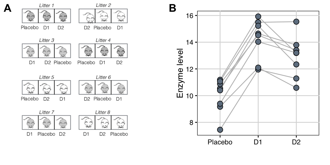
Figure 7.1: Comparing enzyme levels for placebo, D1, and D2 under low fat diet using randomized complete block design. A: Data layout with eight litters of size three, treatments independently randomized in each block. B: Observed enzyme levels for each drug; lines connect responses of mice from the same litter.
7.2.2 Model and Hasse Diagram
Hasse Diagram
Deriving the experiment structure diagram in Figure 7.2C poses no new challenges: the treatment structure contains the single treatment factor Drug with three levels while the unit structure contains the blocking factor (Litter), which groups the units from (Mouse). We consider the specific eight litters in our experiment as a random sample, which makes both unit factors random. The factors Drug and (Litter) are crossed and their combinations are levels of the interaction factor (Litter:Drug); since (Litter) is random, so is the interaction. The randomization allocates levels of Drug on (Mouse), and the experiment structure is similar to a two-way factorial design, but (Litter) originates from the unit structure, is random, and is not randomly allocated to (Mouse), but rather groups levels of (Mouse) by an intrinsic property of each mouse.
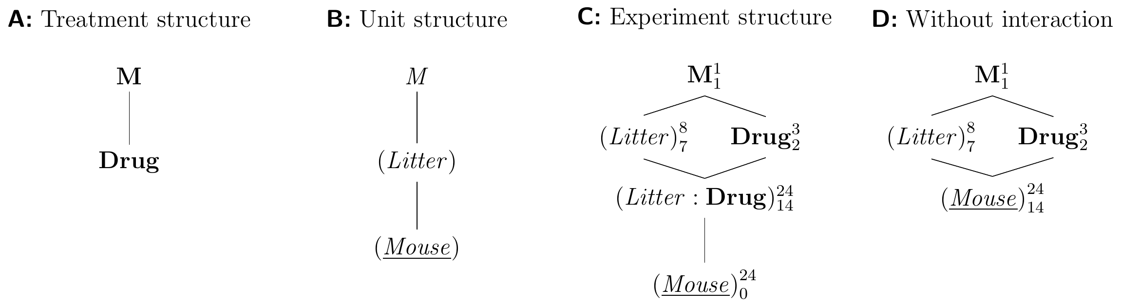
Figure 7.2: Randomized complete block design for determining effect of two different drugs and placebo using eight mice per drug and a single measurement per mouse. Each drug occurs once per block and assignment to mice is randomized independently for each block.
The Block-by-Treatment Interaction
Each treatment occurs only once per block, and the variations due to interactions and residuals are completely confounded. This design is called a randomized complete block design (RCBD). If we want to analyze data from an RCBD, we need to assume that the block-by-treatment interaction is negligible. We can then merge the interaction and residual factors and use the sum of their variation for estimating the residual variance (Fig. 7.2D).
An appreciable block-by-treatment interaction means that the differences in enzyme levels between drugs depend on the litter. Treatment contrasts are then litter-specific and this systematic heterogeneity of treatment effects complicates the analysis and precludes a straightforward interpretation of the results. Such interaction is likely caused by other biologically relevant factors that influence the effect of (some) treatments but that have not been accounted for in our experiment and analysis.
We cannot test the interaction factor and therefore require a non-statistical argument to justify ignoring the interaction. Since we have full control over which property we use for blocking the experimental units, we can often employ subject-matter knowledge to exclude interactions between our chosen blocking factor and the treatment factor. In our particular case, for example, it seems unlikely that the litter affects drugs differently, which justifies treating the litter-by-drug interaction as negligible.
Linear Model
Because the blocking factor levels are random, so are the cell means \(\mu_{ij}\). Moreover, there is a single observation per cell and each cell mean is confounded with the residual for that cell; a two-factor cell means model is therefore not useful for an RCBD.
The parametric model (including block-by-treatment interaction, Fig. 7.2C) is \[ y_{ij} = \mu + \alpha_i + b_j + (\alpha b)_{ij} + e_{ij}\;, \] where \(\mu\) is the grand mean, \(\alpha_i\) the deviation of the average response for drug \(i\) compared to the grand mean, and \(b_j\) is the random effect of block \(j\). We assume that the residuals and block effects are normally distributed as \(e_{ij}\sim N(0,\sigma_e^2)\) and \(b_j\sim N(0,\sigma_b^2)\), and are all mutually independent. The interaction of drug and block effects is a random effect with distribution \((\alpha b)_{ij}\sim N(0,\sigma^2_{\alpha b})\).
For an RCBD, the interaction is completely confounded with the residuals; its parameters \((\alpha b)_{ij}\) cannot be estimated from the experiment without replicating treatments within each block. If interactions are negligible, then \((\alpha b)_{ij}=0\) and we arrive at the additive model (Fig. 7.2D) \[\begin{equation} y_{ij} = \mu + \alpha_i + b_j + e_{ij} \tag{7.1}\;. \end{equation}\] The average response to treatment level \(i\) is then \(\mu_i=\mu+\alpha_i\); its unbiased estimator is \[ \hat{\mu}_i = \frac{1}{b}\sum_{j=1}^b y_{ij}\;, \] with variance \(\text{Var}(\hat{\mu}_i)=(\sigma_b^2+\sigma_e^2)/b\). We then base our contrast analysis on these estimated marginal means, effectively using a cell means model for the treatment factor after correcting for the block effects.
Analysis of Variance
The total sum of squares for the RCBD with an additive model decomposes into sums of squares for each factor involved, such that \[ \text{SS}_\text{tot} = \text{SS}_\text{trt} + \text{SS}_\text{block} + \text{SS}_\text{res}\;, \] and the degrees of freedom decompose accordingly.
The treatment factor is tested using the \(F\)-statistic \[ F = \frac{\text{SS}_\text{trt}/\text{df}_\text{trt}}{\text{SS}_\text{res}/\text{df}_\text{res}}\;, \] and mean squares are formed by dividing each sum of squares by its corresponding degrees of freedom.
For \(k\) treatment factor levels and \(b\) blocks, the test statistic has a \(F_{k-1,\, (b-1)(k-1)}\)-distribution under the omnibus null-hypothesis \(H_0:\mu_1=\mu_2=\cdots =\mu_k\) that all treatment group means are equal. Note that without blocking, the denominator sum of squares would be \(\text{SS}_\text{block} + \text{SS}_\text{res}\) with corresponding loss of power.
We derive the model specification from the Hasse diagrams in Figure 7.2: since fixed and random factors are exclusive to the treatment respectively unit structure, the corresponding terms are 1+drug and Error(litter/mouse); we reduce these terms to drug and Error(litter) and the model is fully specified as y~drug+Error(litter). The analysis of variance table then contains two error strata: one for the block effect and one for the within-block residuals.
We randomized the treatment on the mice within litters, and the within-block variance \(\sigma_e^2\) therefore provides the mean squares for the \(F\)-test denominator; this agrees with the fact that (Mouse) is the closest random factor below Drug in the experiment structure diagram (Fig. 7.2D). The between-block error stratum contains no further factors or tests, since there are no factors randomized on (Litter) in this design. The ANOVA table is then
| Df | Sum Sq | Mean Sq | F value | Pr(>F) | |
|---|---|---|---|---|---|
| Error stratum: Litter | |||||
| Residuals | 7 | 37.08 | 5.3 | ||
| Error stratum: Within | |||||
| drug | 2 | 74.78 | 37.39 | 84.55 | 1.53e-08 |
| Residuals | 14 | 6.19 | 0.44 | ||
The omnibus \(F\)-test for the treatment factor provides clear evidence that the drugs affect the enzyme levels differently and the differences in average enzyme levels between drugs is about 85 times larger than the residual variance.
The effect size \(\eta^2_\text{drug}=\) 63% is large, but measures the variation explained by the drug effects compared to the overall variation, including the variation removed by blocking. It is more meaningful to compare the drug effect to the within-block residuals alone using the partial effect size \(\eta_\text{p, drug}^2=\) 92%, since the litter-to-litter variation is removed by blocking and has no bearing on the precision of the treatment effect estimates. The large effect sizes confirm that the overwhelming fraction of the variation of enzyme levels in each litter is due to the drugs acting differently.
In contrast to a two-way ANOVA with factorial treatment structure, we cannot simplify the analysis to a one-way ANOVA with a single treatment factor with \(b\cdot k\) levels. This is because the blocking factor is random, and the resulting one-way factor would also be a random factor. The omnibus \(F\)-test for this factor is difficult to interpret, and a contrast analysis would be a futile exercise, since we would compare randomly sampled factor levels among each other.
Linear Mixed Model
In contrast to our previous designs, the analysis of an RCBD requires two variance components in our model: the residual within-block variance \(\sigma_e^2\) and the between-block variance \(\sigma_b^2\). The classical analysis of variance handles these by using one error stratum per variance component, but this makes subsequent analyses more tedious. For example, estimates of the two variance components are of direct interest, but while the estimate \(\hat{\sigma}_e^2=\text{MS}_{\text{res}}\) is directly available from the ANOVA result, an estimate for the between-block variance is \[ \hat{\sigma}_b^2 = \frac{\text{MS}_{\text{block}}-\text{MS}_{\text{res}}}{n}\;, \] and requires manual calculation. For our example, we find \(\hat{\sigma}_e^2=\) 0.44 and \(\hat{\sigma}_b^2=\) 1.62 based on the ANOVA mean squares.
An attractive alternative is the linear mixed model, which explicitly considers the different random factors for estimating variance components and parameters of the linear model in Equation (7.1). Linear mixed models offer a very general and powerful extension to linear regression and analysis of variance, but their general theory and estimation are beyond the scope of this book. For our purposes, we only need a small fraction of their possibilities and we use the lmer() function from package lme4 for all our calculations. In specifying a linear mixed model, we use terms of the form (1|X) to introduce a random offset for each level of the factor X; this construct replaces the Error()-term from aov(). The fixed effect part of the model specification remains unaltered. For our example, the model specification is then y~drug+(1|litter), which asks for a fixed effect (\(\alpha_i\)) for each level of Drug, and allows a random offset (\(b_j\)) for each litter.
Fixed effects section of the result gives the parameter estimates for \(\alpha_i\), but they are of secondary interest and depend on the coding (cf. Section 4.7).
| Estimate | Std. Error | df | t value | Pr(>|t|) | |
|---|---|---|---|---|---|
| (Intercept) | 10.01 | 0.51 | 9.4 | 19.73 | 5.73e-09 |
| drugD1 | 4.23 | 0.33 | 14.0 | 12.71 | 4.46e-09 |
| drugD2 | 2.91 | 0.33 | 14.0 | 8.74 | 4.83e-07 |
Random effects section of the result provides the variance and standard deviation for each variance component:
| Group | Name | Variance | Std. Dev. |
|---|---|---|---|
| litter | (Intercept) | 1.62 | 1.27 |
| Residual | 0.44 | 0.67 |
These correspond to the two variance components \(\hat{\sigma}_b^2=\) 1.62 (litter) and \(\hat{\sigma}_e^2=\) 0.44 (Residual), in agreement with the ANOVA results.
We calculate our familiar ANOVA table from an estimated linear mixed model m using anova(m), which yields
| Sum Sq | Mean Sq | NumDF | DenDF | F value | Pr(>F) | |
|---|---|---|---|---|---|---|
| drug | 74.78 | 37.39 | 2 | 14 | 84.55 | 1.53e-08 |
Linear mixed models and ‘traditional’ analysis of variance use the same linear model to analyze data from a given design. Their main difference is the way they handle models with multiple variance components. Analysis of variance relies on the crude concept of error strata, which makes direct estimation of variance more cumbersome and leads to loss in efficiency if information on effects is distributed between error strata (such as in incomplete block designs, discussed in Section 7.3). Linear mixed models use different techniques for estimation of the model’s parameters that make use of all available information. Variance estimates are directly available, and linear mixed models do not suffer from problems with unbalanced group sizes. Colloquially, we can say that the analysis of variance approach provides a convenient framework to phrase design questions, while the linear mixed model provides a more general tool for the subsequent analysis.
7.2.3 Contrasts
In a blocked design with random block factor, the only useful contrasts are between levels of (fixed) treatment factors, since a contrast involving levels of the blocking factor would define a comparison of specific instances of random factor levels. To estimate the difference between the average enzyme level of the first and second litter, for example, only has a useful interpretation if these two arbitrary litters are again used in a replication of the experiment. This is also reflected in the population marginal means, of which there are only three—\(\mu_1,\dots,\mu_3\), one per treatment group—in our example, rather than one per block-treatment combination. We then define and estimate treatment contrasts exactly as before, and briefly exemplify the procedure for our experiment with three contrasts: the comparison of \(D1\) respectively \(D2\) to placebo, and the comparison of the average of \(D1\) and \(D2\) to placebo. The contrasts are \[ \Psi(\mathbf{w}_1) = \mu_2-\mu_1 \,,\quad \Psi(\mathbf{w}_2)=\mu_3-\mu_1 \,,\quad\text{and}\quad \Psi(\mathbf{w}_3)=\frac{\mu_2+\mu_3}{2}-\mu_1\;. \] The following code defines and estimates the contrasts based on the linear mixed model:
# Estimate linear mixed model
lmm.rcbd = lmer(y~drug+(1|litter), data=drugs_litters)
# Estimate group means
em.lmm = emmeans(lmm.rcbd, ~drug)
# Manually define contrasts
psi = list("D1 - Placebo"=c(-1,+1,0),
           "D2 - Placebo"=c(-1,0,+1),
           "(D1+D2)/2 - Placebo"=c(-1,+1/2,+1/2))
# Estimate contrasts
ct.lmm= contrast(em.lmm, psi)
# Get 95%-CI
ci.lmm = confint(ct.lmm)
The contrast estimates for our experiment are shown in Table 7.1 for an analysis based on aov(), the above analysis using lmer(), and an incorrect analysis of variance that ignores the blocking factor and treats the data as coming from a completely randomized design. Ignoring the blocking factor results in a residual variance of \(\sigma_b^2+\sigma_e^2\) instead of \(\sigma_e^2\) for the correct analysis. The resulting decrease in precision is clearly visible.
| Contrast | Estimate | se | df | LCL | UCL |
|---|---|---|---|---|---|
| ANOVA: aov(y~drug+Error(litter)) | |||||
| D1 - Placebo | 4.23 | 0.33 | 14 | 3.51 | 4.94 |
| D2 - Placebo | 2.91 | 0.33 | 14 | 2.19 | 3.62 |
| (D1+D2)/2 - Placebo | 3.57 | 0.29 | 14 | 2.95 | 4.18 |
| Mixed model: lmer(y~drug+(1|litter)) | |||||
| D1 - Placebo | 4.23 | 0.33 | 14 | 3.51 | 4.94 |
| D2 - Placebo | 2.91 | 0.33 | 14 | 2.19 | 3.62 |
| (D1+D2)/2 - Placebo | 3.57 | 0.29 | 14 | 2.95 | 4.18 |
| INCORRECT: aov(y~drug) | |||||
| D1 - Placebo | 4.23 | 0.72 | 21 | 2.73 | 5.72 |
| D2 - Placebo | 2.91 | 0.72 | 21 | 1.41 | 4.40 |
| (D1+D2)/2 - Placebo | 3.57 | 0.62 | 21 | 2.27 | 4.86 |
7.2.4 Evaluating and Choosing a Blocking Factor
Evaluating a Blocking Factor
Once the data are recorded, we are interested in quantifying how ‘good’ the blocking performed in the experiment. This information would allow us to better predict the expected residual variance for a power analysis of our next experiment and to determine if we should continue using the blocking factor.
One way of evaluating the blocking is by treating the blocking factor as fixed, and specify the ANOVA model as y~drug+litter. The ANOVA table then contains a row for the blocking factor with an associated \(F\)-test (Samuels, Casella, and McCabe 1991). This test only tells us if the between-block variance is significantly different from zero, but does not quantify the advantage of blocking.
A more meaningful alternative is the calculation of appropriate effect sizes, and we can determine the percentage of variation removed from the analysis by blocking using the effect size \(\eta^2_\text{block}\), which evaluates to 31% for our example. In addition, the partial effect \(\eta^2_\text{p, block}=\) 86% shows that the vast majority of non-treatment sum of squares is due to the litter-to-litter variation and blocking by litter was a very successful strategy.
Alternatively, the intraclass correlation coefficient \(\text{ICC}=\sigma_b^2 / (\sigma_b^2+\sigma_e^2)\) uses the proportion of variance and we find an ICC of 79% for our example, confirming that the blocking works well. The ICC is directly related to the relative efficiency of the RCBD compared to a non-blocked CRD, since \[\begin{equation} \text{RE}(\text{CRD},\text{RCBD}) = \frac{\sigma_b^2+\sigma_e^2}{\sigma_e^2} = \frac{1}{1-\text{ICC}} \tag{7.2} \;, \end{equation}\] and \(\sigma_b^2+\sigma_e^2\) is the residual variance of a corresponding CRD. From our estimates of the variance components, we find a relative efficiency of 4.66; to achieve the same precision as our blocked design with 8 mice per treatment group would require about 37 mice per treatment group for a completely randomized design.
We can alternatively find the relative efficiency as \[ \text{RE}(\text{CRD},\text{RCBD}) = \frac{\widehat{\text{MS}}_\text{res, CRD}}{\text{MS}_\text{res, RCBD}}\;, \] where we estimate the residual mean squares of the CRD from the ANOVA table of the RCBD as a weighted average of the block and the residual sums of squares, weighted by the corresponding degrees of freedom: \[ \widehat{\text{MS}}_\text{res, CRD} = \frac{\text{df}_\text{block}\cdot \text{MS}_\text{block}\, +\, (\text{df}_\text{trt}+\text{df}_\text{res})\cdot \text{MS}_\text{res}}{\text{df}_\text{block}+\text{df}_\text{trt}+\text{df}_\text{res}}\;. \] For our example, \(\widehat{\text{MS}}_\text{res, CRD}=\) 1.92, resulting in a relative efficiency estimate of RE(CRD,RCBD)=4.34. It differs slightly from our previous estimate because it uses an approximation based on the ANOVA results rather than estimates of the variance components based on the linear mixed model.
Choosing a Blocking Factor
The main purpose of blocking is to decrease the residual variance for improving the power of tests and precision of estimates by grouping the experimental units before the allocation of treatments, such that units within the same block are more similar than units from different blocks. The blocking factor must therefore describe a property of experimental units that affects all treatments equally to avoid a block-by-treatment interaction, and that is independent of the treatment outcome, which precludes, e.g., grouping ‘responders’ and ‘non-responders’ based on the measured response.
Some examples of grouping units using intrinsic properties are (i) litters of animals; (ii) parts of a single animal or plant, such as left/right kidney or leafs; (iii) initial weight; (iv) age or co-morbidities; (v) biomarker values, such as blood pressure, state of tumor, or vaccination status. Properties non-specific to the experimental units include (i) batches of chemicals used for the experimental unit; (ii) device used for measurements; or (iii) date in multi-day experiments. These are often necessary to account for systematic differences from the logistics of the experiment (such as batch effects); they also increase the generalizability of inferences due to the broader experimental conditions.
The golden rule for designing experiments with blocks is
Block what you can, randomize what you can not.
As always, practical considerations should be taken into account when deciding upon blocking and randomization. There is no point in designing an overly complicated blocked experiment that becomes too difficult to implement correctly. On the other hand, there is no harm if we use a blocking factor that turns out to have no or minimal effect on the residual variance.
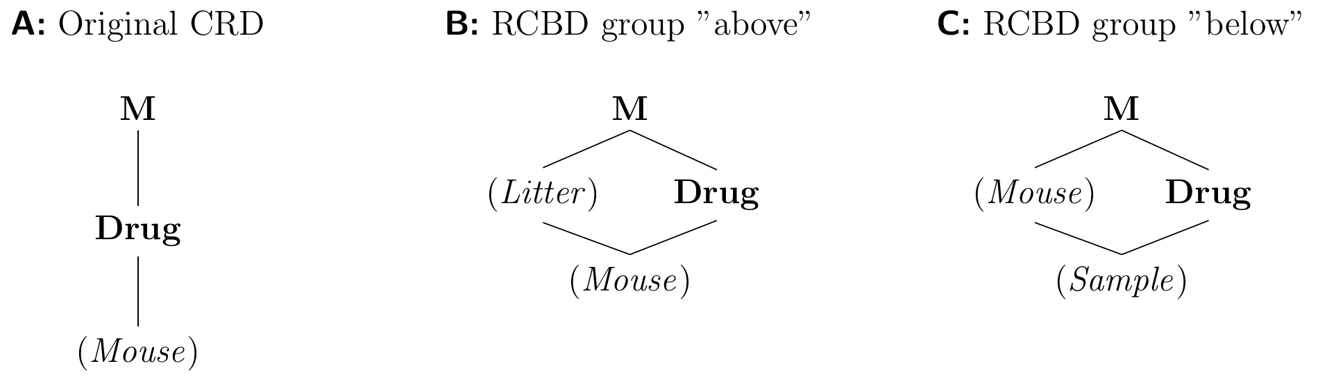
Figure 7.3: Creating a randomized complete block design from a completely randomized design. A: A CRD randomizes drugs on mice. B: Introducing a blocking factor ‘above’ groups the experimental units. C: Subdividing each experimental units and randomizing the treatments on the lower level creates a new experimental unit factor ‘below.’
We can think about creating a blocked design by starting from a completely randomized design and ‘splitting’ the experimental unit factor into a blocking and a nested (potentially new) unit factor. Two examples are shown in Figure 7.3, starting from the CRD (Figure 7.3A) randomly allocating drug treatments on mice. In the first RCBD (Figure 7.3B), we create a blocking factor ‘above’ the original experimental unit factor and group mice by their litters. This restricts the randomization of Drug to mice within litters. In the second RCBD (Figure 7.3C), we subdivide the experimental unit into smaller units by taking multiple samples per mouse. This re-purposes the original experimental unit factor as the blocking factor and introduces a new factor ‘below,’ but requires that we now randomize Drug on (Sample) to obtain an RCBD and not pseudo-replication.
7.2.5 Power Analysis and Sample Size
Power analysis for a randomized complete block design with no block-by-treatment interaction is very similar to a completely randomized design, the only difference being that we use the within-block variance \(\sigma_e^2\) as our residual variance. For a main effect with parameters \(\alpha_i\), the noncentrality parameter is thus \(\lambda_R=n\sum_i \alpha_i^2/\sigma_e^2=n\cdot k\cdot f_R^2\), while it is \(\lambda_C=n\sum_i \alpha_i^2/(\sigma_b^2+\sigma_e^2)=n\cdot k \cdot f_C^2\) for the same treatment structure in a completely randomized design. The two effect sizes are different for the same raw effect size, and \(f_C^2\) is smaller than \(f_R^2\) for the same values of \(n\), \(k\), and \(\alpha_i\); this directly reflects the increased precision in an RCBD.
The denominator degrees of freedom are \((k-1)(b-1)=kb-k-(b-1)\) for an RCBD and we loose \(b-1\) degrees of freedom compared to the \(k(b-1)=kb-k\) degrees of freedom for a CRD. The corresponding loss in power is very small and more than compensated by the simultaneous increase in power due to the smaller residual variance unless the blocking is very ineffective and the number of blocks large.
As an example, we consider a single treatment factor with \(k=\) 3 levels, a total sample size of \(N=b\cdot k=\) 30, and an effect size of \(f_{C,0}^2=\) 0.0625 for the treatment main effect at a significance level of \(\alpha=5\%\). The residual variance is \(\sigma^2=\) 2. Under a completely randomized design, we have a power of 20% for detecting the effect. This power increases dramatically to 61% when we organize the experimental units into \(b=\) 10 blocks with between-block variance \(\sigma_b^2=\) 1.5 and within-block variance \(\sigma_e^2=\) 0.5. The much smaller residual variance increases the standardized effect size to \(f_{R,0}^2=(\sigma_b^2+\sigma_e^2)/\sigma_e^2\cdot f^2_{C,0}=\) 0.25; the increase is exactly the relative efficiency (Eq. (7.2)).
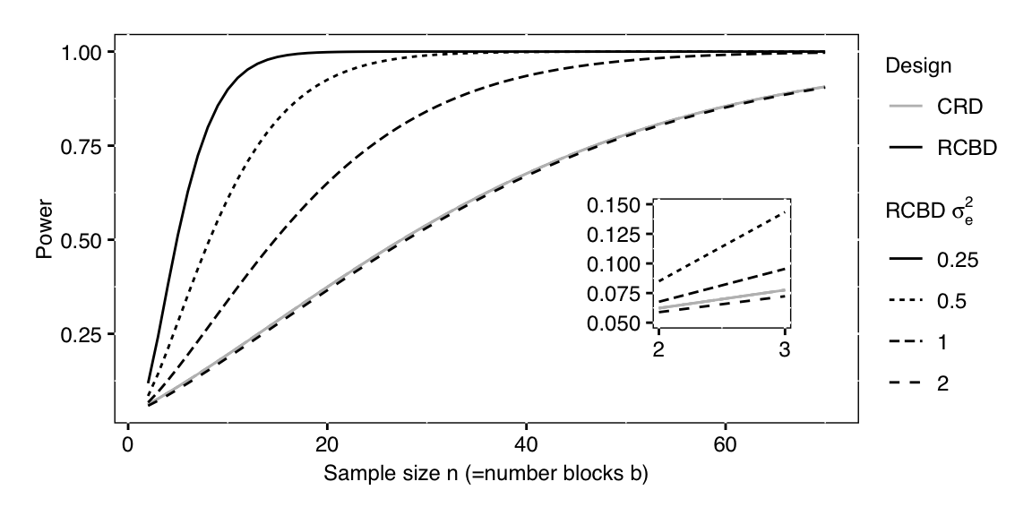
Figure 7.4: Power for different sample sizes n for a completely randomized design with residual variance two and four randomized complete block designs with same overall variance, but four different within-block residual variances. Inset: same curves for small sample sizes show lower power of RCBD than CRD for identical residual variance due to lower residual degrees of freedom in the RCBD.
The relation between power and within-block variance is shown in Figure 7.4 for five scenarios with significance level \(\alpha=5\%\) and an omnibus-\(F\) test for a main effect with \(k=\) 3 treatment levels. The solid grey curve shows the power for a CRD with residual variance \(\sigma_e^2+\sigma_b^2=2\) as a function of sample size per group and a minimal detectable effect size of \(f^2_\text{C}=\) 0.0625. The black curves show the power for an RCBD with four different within-block variances from \(\sigma_e^2=0.25\) to \(\sigma_e^2=2\). For the same sample size, the RCBD then has larger effect size \(f^2_\text{R}\), which translates into higher power. The inset figure shows that an RCBD has negligibly less power than a CRD for the same residual variance of \(\sigma_e^2=2\), due to the loss of \(b-1\) degrees of freedom.
7.2.6 Replication Within Blocks
Within-block replication by using each treatment multiple times in each block is usually not a profitable strategy, and we should increase replication in an RCBD by introducing more blocks. A rare exception occurs when the blocking factor is not very efficient or measurement error is large, and the residual variance \(\sigma_e^2\) is large compared to the between-block variance \(\sigma_b^2\). Observing each treatment multiple times per block might then increase the precision of within-block contrast estimates.
In some scenarios, however, it is necessary to use more than one replicate of each treatment per block. This is typically the case if our blocking factor is non-specific and introduced to capture grouping due to the logistics of the experiment. For example, we might conduct our drug comparisons in two different laboratories. We then replicate a full CRD in the two laboratories, leading to a design with (Lab) as a blocking factor, but multiple observations of each treatment in each laboratory. This design is helpful to account for laboratory-specific differences.
Another purpose for using a multi-laboratory experiment is to broaden the inference for our experiment. If we find stable estimates of contrasts between laboratories despite the expected systematic differences, then we demonstrated experimentally that our scientific findings are independent of ‘typical’ alterations in the protocol or chemicals used, for example.
The resulting design is called a generalized randomized complete block design (GRCBD) and its diagrams are shown in Figure 7.5 for eight mice per drug and two laboratories
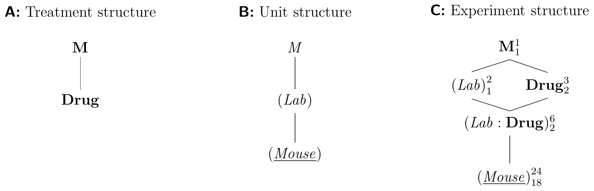
Figure 7.5: A (generalized) randomized complete block design (GRCBD) with four mice per drug and laboratory. Completely randomized design for estimating drug effects of three drugs replicated in two laboratories.
Each mouse is used in exactly one laboratory and (Lab) thus groups (Mouse). We use the same drugs in both laboratories, making (Lab) and Drug crossed factors. The replication of treatments in each block allows estimation of the lab-by-drug interaction, which provides information about the stability of the effects and contrasts. The linear model with interaction is
\[
y_{ijk} = \mu + \alpha_i + b_j + (\alpha b)_{ij} + e_{ijk}\;,
\]
where \(\alpha_i\) are the (fixed) treatment effect parameters, \(b_j\) the random block effect parameters with \(b_j\sim N(0,\sigma_b^2)\), \((\alpha b)_{ij}\sim N(0,\sigma_{\alpha b}^2)\) describes the interaction of treatment \(i\) and laboratory \(j\), and \(e_{ijk}\sim N(0,\sigma_e^2)\) are the residuals. The specification for a linear mixed model is y ~ drug + (1|lab) + (1|lab:drug) for our example.
If the lab-by-treatment interaction is negligible with \(\sigma_{\alpha b}^2\approx 0\), we remove the interaction term from the analysis and arrive at the additive model. Then, (Lab) acts as a blocking factor just like (Litter) in the previous example and eliminates the lab-to-lab variation from treatment contrasts.
If the interaction is appreciable and cannot be neglected, then the contrasts between drugs are different between the two labs, and we cannot determine generalizable drug effects. Now, (Lab:Drug) is the first random factor below Drug and provides the factor for comparing levels of Drug, and (Mouse) is sub-sampled from (Lab:Drug). Consequently, the variation against which drug effects are tested is larger and replication is lower, leading to decrease in precision and power for treatment contrasts.
7.2.7 Fixed Blocking Factors
We can typically consider the levels of a blocking factor as randomly drawn from a set of potential levels. The blocking factor is then random, and we are not interested in contrasts involving its levels, for example, but rather use the blocking factor to increase precision and power by removing parts of the variation from treatment contrasts.
A typical example of a non-random classification factor is the sex of an animal. The Hasse diagrams in Figure 7.6 show an experiment design to study the effects of our three drugs on both female and male mice. Each treatment group has eight mice, with half of them female, the other half male. The experiment design looks similar to a factorial design of Chapter 6, but the interpretation of its analysis is rather different. Most importantly, while the factor Sex is fixed with only two possible levels, its levels are not randomly assigned to mice. This is reflected in the fact that Sex groups mice by an intrinsic property and hence belongs to the unit structure. In contrast, levels of Drug are randomly assigned to mice, and Drug therefore belongs to the treatment structure of the experiment.
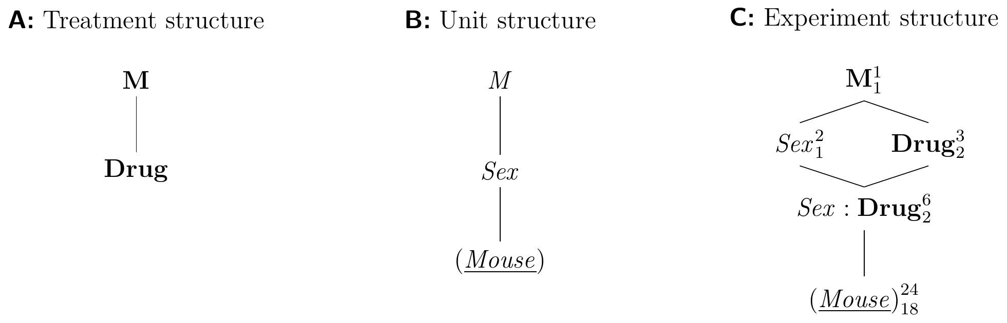
Figure 7.6: A blocked design using sex of mouse as a fixed classification factor, with four female and four male mice in of three each treatment groups.
In contrast to a randomized complete block design, we cannot increase the number of blocks to increase the replication. With two levels of Sex fixed, we instead need to increase the experiment size by using multiple mice of each sex for each drug. Since Sex and Drug are fixed, so is their interaction, and all fixed factors are tested against the same error term from (Mouse).
The specification for the analysis of variance is y~drug*sex, and it looks exactly like the specification of a two-way ANOVA. However, since Sex is a unit factor that is not randomized, the roles of Sex and Drug are not symmetric and the interpretation is rather different from our previous two-way ANOVA with treatment factors Drug and Diet. In the factorial design, the presence of a Drug:Diet interaction means that we can modify the effect of a drug by using a different diet. In the fixed-block design, a Sex:Drug interaction means that the effect of drugs is not stable over the sexes and some drugs affect female and male mice differently. We can use a drug to alter the enzyme level in a mouse, but we cannot alter the sex of that mouse to modulate the drug effect.
7.2.8 Factorial Treatment Structure
It is straightforward to extend an RCBD from a single treatment factor to factorial treatment structures by crossing the entire treatment structure with the blocking factor. Each block then contains one full replicate of the factorial design, and the required block size rapidly increases with the number of factors and factor levels. In practice, only smaller factorials can be blocked by this method since heterogeneity between experimental units often increases with block size, diminishing the advantages of blocking. We discuss more sophisticated designs for blocking factorials that overcome this problem by using only a fraction of all treatment combinations per block in Chapter 9.
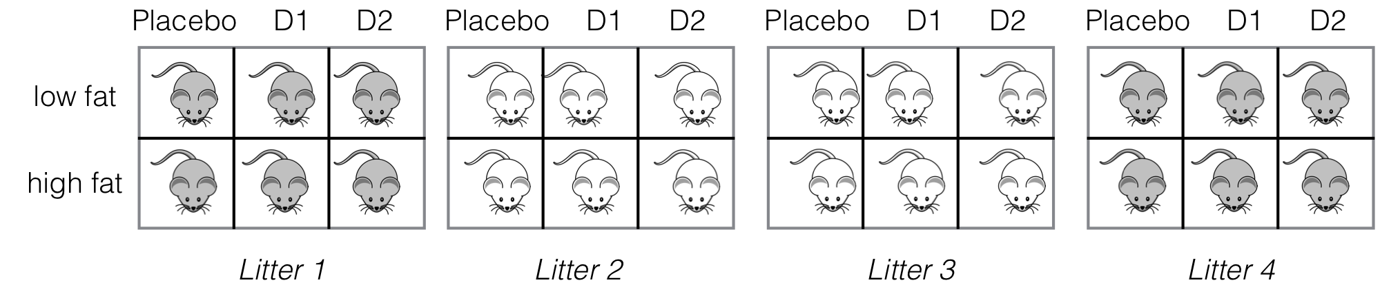
Figure 7.7: Experiment layout for three drugs under two diets, four litter blocks. Two-way crossed treatment structure within each block.
We illustrate the extension using our drug-diet example from Chapter 6 where three drugs were combined with two diets. The six treatment combinations can still be accommodated when blocking by litter, and using four litters of size six results in the experimental layout shown in Figure 7.7 with 24 mice in total. Already including a medium-fat diet would require atypical litter sizes of nine mice, however.
Model and Hasse Diagram
For constructing the Hasse diagrams in Figure 7.8 we note that the blocking factor is crossed with the full treatment structure—both treatment factors and the treatment interaction factor. We assume that our blocking factor does not differentially change the diet or drug effects and consequently ignore all three block-by-treatment interactions (Litter:Diet), (Litter:Drug), and (Litter:Diet:Drug).
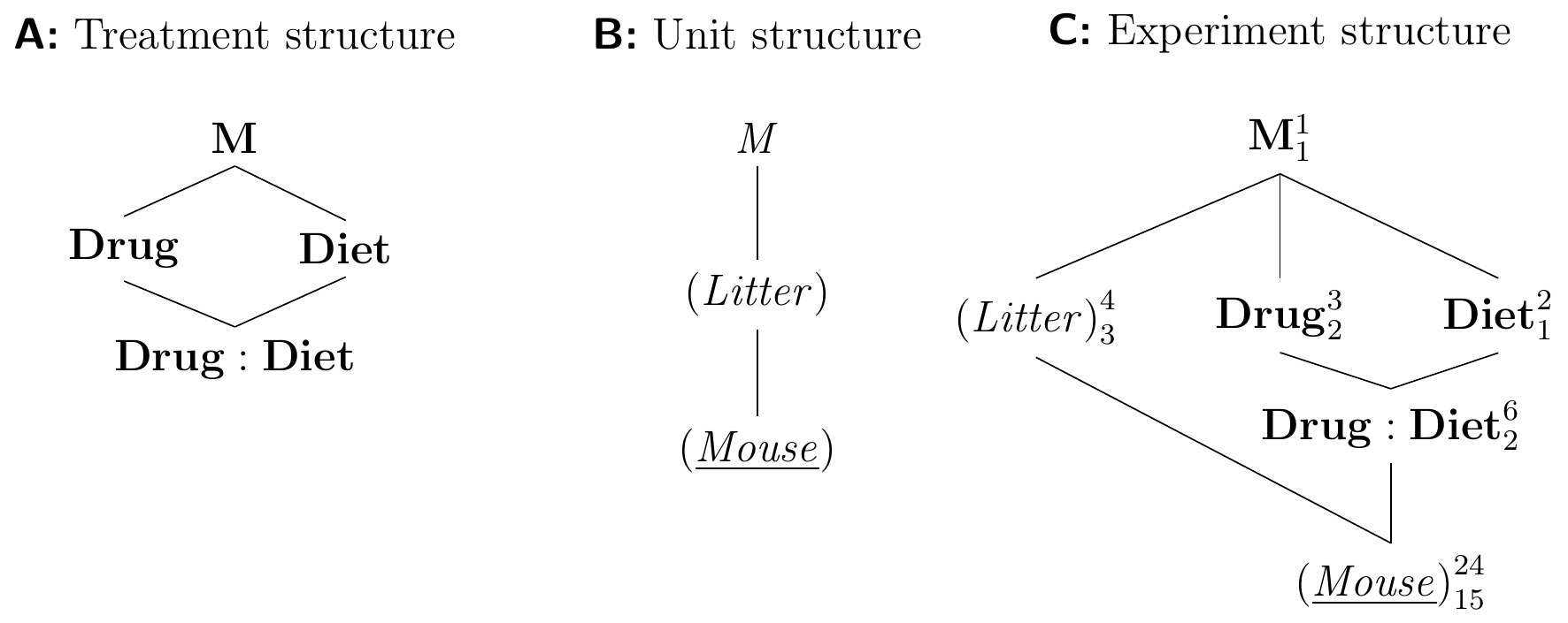
Figure 7.8: Randomized complete block design for determining effect of two different drugs and placebo combined with two different diets using four mice per drug and diet, and a single response measurement per mouse. All treatment combinations occur once per block and are randomized independently.
We can easily derive a corresponding linear model from the Hasse diagrams. It is identical to our ‘usual’ model for an RCBD, except that its mean structure additionally contains the parameters for the second treatment factor and the interaction: \[ y_{ijk} = \mu + \alpha_i + \beta_j + (\alpha\beta)_{ij} + b_k + e_{ijk}\;, \] where \(\alpha_i\) and \(\beta_j\) are the main effects of drug and diet, respectively, \((\alpha\beta)_{ij}\) the interaction effects between them, \(b_k\sim N(0,\sigma_b^2)\) are the random block effects, and \(e_{ijk}\sim N(0,\sigma_e^2)\) are the residuals. Again we assume that all random effects are mutually independent.
The enzyme levels \(y_{ijk}\) are shown in Figure 7.9 as dark grey points in an interaction plot separately for each block. We can clearly see the block effects, which systematically shift enzyme levels for all conditions. After estimating the linear model, the shift \(b_k\) can be estimated for each block, and the light grey points show the resulting ‘normalized’ data \(y_{ijk}-\hat{b}_k\) after accounting for the block effects.
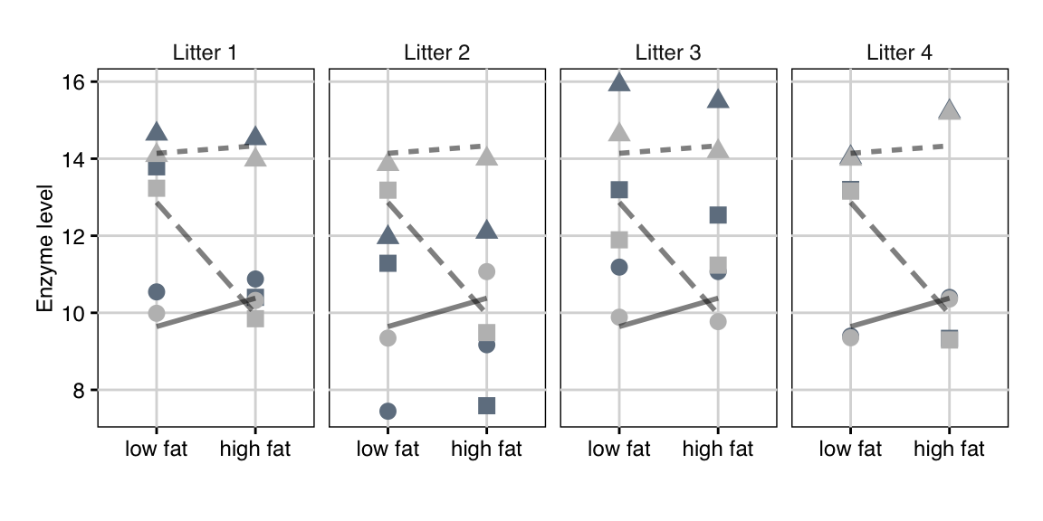
Figure 7.9: Enzyme levels for placebo (point), drug D1 (triangle), and drug D2 (square). Data are shown separately for each of four litters (blocks). Lines connect mean values over litters of same drug under low and high fat diets. Dark grey points are raw data, light grey points are enzyme levels adjusted for block effect.
ANOVA Table
We analyze the resulting data using either analysis of variance or a linear mixed model. The two model specifications derive directly from the Hasse diagrams and consist of two main effects and interaction for the treatment factors and an error stratum respectively random intercept for the litter unit factor. The specifications are y~drug*diet+Error(litter), respectively y~drug*diet+(1|litter).
The resulting ANOVA table based on the linear mixed model is
| Sum Sq | Mean Sq | NumDF | DenDF | F value | Pr(>F) | |
|---|---|---|---|---|---|---|
| drug | 74.1 | 37.05 | 2 | 15 | 91.54 | 3.93e-09 |
| diet | 2.59 | 2.59 | 1 | 15 | 6.39 | 2.32e-02 |
| drug:diet | 15.41 | 7.71 | 2 | 15 | 19.04 | 7.65e-05 |
Blocking by litter reduces the residual variance from 1.19 for the non-blocked design in Chapter 6 to 0.64, the relative efficiency is RE(CRD,RCBD)= 1.87. Due to the increase in power, the Diet main effect is now significant.
Contrasts
The definition and analysis of linear contrasts work exactly as for the two-way ANOVA in Section 6.6, and contrasts are defined on the six treatment group means. For direct comparison with our previous results, we estimate the two interaction contrasts of Table 6.6 in the blocked design. They compare the difference in enzyme levels for D1 (resp. D2) under low and high fat diet to the corresponding difference in the placebo group; estimates and Bonferroni-corrected confidence intervals are shown in Table 7.2.
| Contrast | Estimate | se | df | LCL | UCL |
|---|---|---|---|---|---|
| (D1 low - D1 high) - (Pl. low - Pl. high) | 0.54 | 0.64 | 15 | -1.04 | 2.13 |
| (D2 low - D2 high) - (Pl. low - Pl. high) | 3.64 | 0.64 | 15 | 2.06 | 5.22 |
As expected, the estimates are similar to those we found previously, but confidence intervals are substantially narrower due to the increase in precision.
7.3 Incomplete Block Designs
7.3.1 Introduction
The randomized complete block design can be too restrictive if the number of treatment levels is large or the available block sizes small. Fractional factorial designs offer a solution for factorial treatment structures by confounding some treatment effects with blocks (Chapter 9). For a single treatment factor, we can use incomplete block designs (IBD), where we deliberately relax the complete balance of the previous designs and use only a subset of the treatments in each block.
The most important example is the balanced incomplete block design (BIBD), where each pair of treatments is allocated to the same number of blocks, and so are therefore all individual treatments. This specific type of balance ensures that pair-wise contrasts are all estimated with the same precision, but precision decreases if more than two treatment groups are compared.
We illustrate this design with our drug example, where three drug treatments are allocated to 24 mice on a low fat diet. If the sample preparation is so elaborate that only two mice can be measured at the same time, then we have to run this experiment in twelve batches, with each batch containing one of three treatment pairs: (placebo, \(D1\)), (placebo, \(D2\)), or (\(D1\), \(D2\)). A possible balanced incomplete block design is shown in Figure 7.10, where each treatment pair is used in four blocks, and the treatments are randomized independently to mice within each block. The resulting data are shown in Table 7.3.
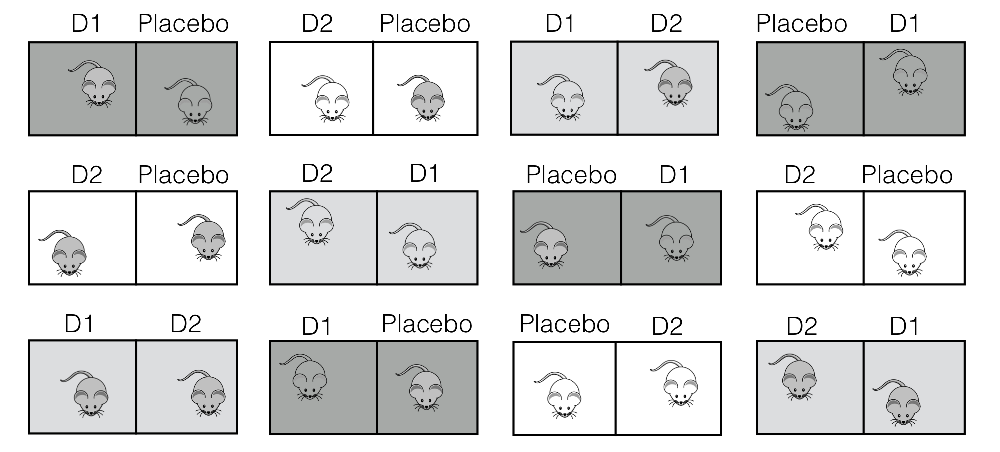
Figure 7.10: Experiment layout for a balanced incomplete block design with three drugs in twelve batches of size two.
|
|
|
7.3.2 Defining a Balanced Incomplete Block Design
The key requirement of a BIBD is that all pairs of treatments occur the same number of times in a block. This requirement restricts the possible combinations of number of treatments, block size, and number of blocks. With three pairs of treatments as in our example, the number of blocks in a BIBD is restricted to be a multiple of three. The relations between the parameters of a BIBD are known as the two defining equations \[\begin{equation} rk = bs \quad\text{and}\quad \lambda\cdot (k-1) = r\cdot (s-1)\;. \tag{7.3} \end{equation}\] They relate the number of treatments \(k\), number of blocks \(b\), block size \(s\) to the number of times \(r\) that each treatment occurs and the number of times \(\lambda\) that each pair of treatments occurs in the same block. If these equations hold, then the corresponding design is a BIBD.
The equations are derived as follows: with \(b\) blocks of \(s\) units each, the product \(bs\) is the total number of experimental units in the experiment. This number has to equal \(rk\), since each of the \(k\) treatments occurs in \(r\) blocks. Moreover, each particular treatment occurs \(\lambda\) times with each of the remaining \(k-1\) treatments. It also occurs in \(r\) blocks, and is combined with \(s-1\) other treatments in each block.
For our example, we have \(k=3\) treatment levels and each treatment occurs in \(r=8\) blocks, we have \(b=12\) blocks each of size \(s=2\), resulting in \(\lambda=4\) co-occurrences of each pair in the same block. This satisfies the defining equations and our design is a BIBD. In contrast, for only \(b=5\) blocks, we are unable to satisfy the defining equations and no corresponding BIBD exists.
In order to generate a balanced incomplete block design, we need to find parameters \(s\), \(r\), and \(\lambda\) such that the defining equations (7.3) hold. A particularly simple way is by generating an unreduced or combinatorial design and use as many blocks as there are ways to select \(s\) out of \(k\) treatment levels. The number of blocks \(b\) is then \(b={k \choose s}=k!/(k-s)!s!\) and increases rapidly with \(k\).
We can often improve on the unreduced design, and generate a valid BIBD with substantially fewer blocks. Experimental design books sometimes contain tables of BIBDs for different number of treatment and block sizes, see for example Cochran and Cox (1957). As a further example, we consider constructing a BIBD for \(k=6\) treatments in blocks of size \(s=3\). The unreduced combinatorial design requires \(b={6 \choose 3}=20\) blocks (experiment size \(N=60\)). Not all of these are needed to fulfill the defining equations, however, and a smaller BIBD exists with only \(b=10\) blocks (and \(N=30\)).
7.3.3 Analysis
The balanced incomplete block design is not fully balanced: since only a fraction of the available treatment levels occur in each block, some combinations of block and treatment levels are not observed, resulting in some-cells-empty data. The treatment and block main effects are no longer independent, but the requirements encoded in the two defining equations ensure that unbiased estimates exist for all treatment effects, and that standard ANOVA techniques are available for the analysis. However, the treatment and block factor sums of squares are not independent, and while their sum remains the same, their individual values now depend on the order of the two factors in the model specification. Moreover, part of the information about treatment effects is captured by the differences in blocks; in particular, there are two omnibus \(F\)-tests for the treatment factor, the first based on the inter-block information and located in the ANOVA table in the block-factor error stratum, and the second based—as for an RCBD—on the intra-block information and located in the residual error stratum. A linear mixed model automatically combines these information, and analysis of variance and mixed model results no longer concur exactly for a BIBD.
Linear Model
If we assume negligible block-by-treatment interaction, the linear model for a balanced incomplete block design is the additive model \[ y_{ij} = \mu + \alpha_i + b_j + e_{ij}\;, \] where \(\mu\) is the grand mean, \(\alpha_i\) the expected difference between the group mean for treatment \(i\) and the grand mean, \(b_j\sim N(0,\sigma_b^2)\) are the random block effects, and \(e_{ij}\sim N(0,\sigma_e^2)\) are the residuals. All random variables are mutually independent.
Not all block-treatment combinations occur in a BIBD, and some of the \(y_{ij}\) therefore do not exist. As a consequence, naive parameter estimators are biased, and more complex estimators are required for the parameters and treatment group means. We forego a more detailed discussion of these problems and rely on statistical software like R to provide appropriate estimates for BIBDs.
Intra- and Inter-block Information
In an RCBD, we can estimate any treatment contrast and all effects independently within each block, and then average over blocks. We can use the same intra-block analysis for a BIBD by estimating contrasts and effects based on those blocks that contain sufficient information and averaging over these blocks. The resulting estimates are free of block effects.
In addition, the block totals—calculated by adding up all response values in a block—also contain information about contrasts and effects if the block factor is random. This information can be extracted by an inter-block analysis. We again refrain from discussing the technical details, but provide some intuition for the recovery of inter-block information.
We consider our example with three drugs in blocks of pairs and are interested in estimating the average enzyme level under the placebo treatment. Using the intra-block information, we would adjust each response value by the block effect, and average over the resulting adjusted placebo responses. For the inter-block analysis, first note that the true treatment group means are \(\mu+\alpha_1\), \(\mu+\alpha_2\), and \(\mu+\alpha_3\) for placebo, \(D1\), and \(D2\), respectively. The block totals for the three types of block are then (placebo, \(D1\))\(=T_{P,D1}=\mu+\alpha_1+\mu+\alpha_2\), (placebo, \(D2\))\(=T_{P,D2}=\mu+\alpha_1+\mu+\alpha_3\), and (\(D1\), \(D2\))\(=T_{D1,D2}=\mu+\alpha_2+\mu+\alpha_3\), respectively and each type of block occurs the same number of times.
The treatment group mean for placebo can then be calculated from the block totals as \((T_{P,D1}+T_{P,D2}-T_{D1,D2})/2\), since \[\begin{align*} \frac{T_{P,D1}+T_{P,D2}-T_{D1,D2}}{2} &= \frac{2\mu+\alpha_1+\alpha_2}{2} + \frac{2\mu+\alpha_1+\alpha_3}{2} - \frac{2\mu+\alpha_2+\alpha_3}{2} \\ &=\frac{\left(4\mu+2\alpha_1+\alpha_2+\alpha_3\right) - \left(2\mu+\alpha_2+\alpha_3\right)}{2} = \mu+\alpha_1. \end{align*}\] In our illustration (Fig. 7.10), this corresponds to taking the sum over responses in the white and dark grey blocks, and subtracting the responses in the light grey blocks. Note that no information about treatment effects is contained in the block totals of an RCBD.
Analysis of Variance
Based on the linear model, the specification for the analysis of variance isy~drug+Error(block) for a random block factor, the same as for an RCBD. The resulting ANOVA table has again two error strata, and the block error stratum contains the inter-block information about the treatment effects. With two sums of squares, the analysis provides two different omnibus \(F\)-tests for the treatment factor.
| Df | Sum Sq | Mean Sq | F value | Pr(>F) | |
|---|---|---|---|---|---|
| Error stratum: Batch | |||||
| drug | 2 | 14.82 | 7.41 | 3.42 | 7.88e-02 |
| Residuals | 9 | 19.53 | 2.17 | ||
| Error stratum: Within | |||||
| drug | 2 | 56.3 | 28.15 | 98.06 | 2.69e-07 |
| Residuals | 10 | 2.87 | 0.29 | ||
The first \(F\)-test is based on the inter-block information about the treatment, and is in general (much) less powerful than the second \(F\)-test based on the intra-block information. Both \(F\)-tests can be combined to an overall \(F\)-test taking account of all information, but the inter-block \(F\)-test is typically ignored in practice and only the intra-block \(F\)-test is used and reported; this approximation leads to a (often small) loss in power.
The dependence of the block- and treatment factors must be considered for fixed block effects. The correct model specification contains the blocking factor before the treatment factor in the formula, and is y~block+drug for our example. This model adjusts treatments for blocks and the analysis is identical to an intra-block analysis for random block factors. The model y~drug+block, on the other hand, yields an entirely different ANOVA table and an incorrect \(F\)-test, as we discussed in Section 6.5.
Linear Mixed Model
The linear mixed model approach does not require error strata to cope with the two variance components, and provides a single estimate of the drug effects and treatment group means based on all available information. The resulting degrees of freedom are no longer integers and resulting \(F\)-tests and \(p\)-values can deviate from the classical analysis of variance. We specify the model as y~drug+(1|block); this results in the ANOVA table
| Sum Sq | Mean Sq | NumDF | DenDF | F value | Pr(>F) | |
|---|---|---|---|---|---|---|
| drug | 57.23 | 28.62 | 2 | 10.74 | 99.33 | 1.19e-07 |
We note that the sum of squares and the mean square estimates are slightly larger than for the aov() analysis, because the between-block information is taken into account. This provides more power and results in a slightly larger value of the \(F\)-statistic.
This is an example of a design in which the deliberate violation of complete balance still allows an analysis of variance, but where a mixed model analysis gives advantages both in the calculation but also the interpretation of the results. Since the BIBD is not fully balanced, the linear mixed model ANOVA table gives slightly different results when we approximate degrees of freedom with the more conservative Kenward-Roger method rather than the Satterthwaite method reported here.
7.3.4 Contrasts
Contrasts are defined exactly as for our previous designs, but their estimation is based only on the intra-block information if the estimated marginal means are calculated from the ANOVA model. Estimates and confidence intervals then differ between ANOVA and linear mixed model results, and the latter should be preferred. For our example, we calculate three contrasts comparing each drug respectively their average to placebo. The results are given in Table 7.4, and demonstrate the differences in degrees of freedom and precision between the two underlying models.
| Contrast | Estimate | se | df | LCL | UCL |
|---|---|---|---|---|---|
| ANOVA: aov(y~drug+Error(block)) | |||||
| D1 - Placebo | 4.28 | 0.31 | 10.00 | 3.59 | 4.97 |
| D2 - Placebo | 2.70 | 0.31 | 10.00 | 2.01 | 3.39 |
| (D1+D2)/2 - Placebo | 3.49 | 0.27 | 10.00 | 2.90 | 4.09 |
| Mixed model: lmer(y~drug+(1|block)) | |||||
| D1 - Placebo | 4.22 | 0.31 | 10.81 | 3.54 | 4.90 |
| D2 - Placebo | 2.74 | 0.31 | 10.81 | 2.06 | 3.42 |
| (D1+D2)/2 - Placebo | 3.48 | 0.27 | 10.81 | 2.89 | 4.07 |
Estimation of all treatment contrasts is unbiased and contrast variances are free of the block variance in a BIBD. The variance of a contrast estimate is \[ \text{Var}(\hat{\Psi}(\mathbf{w})) = \frac{s}{\lambda k}\sigma_e^2\sum_{i=1}^kw_i^2\;. \] where each treatment is assigned to \(r\) units. The corresponding contrast in an RCBD with the same number \(n=r\) of replicates for each treatment (but lower number of blocks) has variance \(\sigma_e^2\sum_i w_i^2/n\).
We can interpret the term \[ \frac{\lambda k}{s}=r\frac{k}{s}\frac{s-1}{k-1}=n^* \] as the “effective sample size” in each treatment group for a BIBD. It is smaller than the actual replication \(r\) since some information is lost as we cannot fully eliminate the block variances from the group mean estimates.
The relative efficiency of a BIBD compared to an RCBD with \(r\) blocks is \[ \text{RE}_{\Psi}(\text{BIBD},\text{RCBD}) = \frac{r\frac{k}{s}\frac{s-1}{k-1}}{r} = \frac{n^*}{r}\;. \] The fewer treatments fit into a single block, the lower the relative efficiency. For our example, \(k=3\) and \(s=2\) result in a relative efficiency of \(3/4\), and our BIBD requires about 33% more samples to achieve the same precision as an RCBD.
7.3.5 A Real-Life Example—Between-Plates Variability
As a real-world application, we consider an experiment to characterize and compare multiple antibody assays. Each assay only requires a small amount of patient serum, and in order to provide sufficient sample size for precisely estimating the sensitivity and specificity of each assay, several hundred patient samples were used. The samples were distributed over ten 96-well plates, and one concern was the reproducibility of results between plates, since each plate might be handled by a different technician and time between preparing the plate and pipetting each sample onto the assays might vary. For estimating between-plate variability, we would ideally create ten aliquots from several patient sera, and assign one aliquot to each plate. However, the available sera only allowed at most five aliquots of sufficient volume. In this experiment, we are interested in contrasting the plates on the same patients, not the patients themselves. The ten plates are then the treatment factor levels, and each patient is a block to which we assign plates.
| Aliquot | 1 | 2 | 3 | 4 | 5 | 6 | 7 | 8 | 9 | 10 | 11 | 12 | 13 | 14 | 15 | 16 | 17 | 18 |
|---|---|---|---|---|---|---|---|---|---|---|---|---|---|---|---|---|---|---|
| 1 | D | D | E | E | J | J | C | H | E | B | J | F | I | B | E | G | A | J |
| 2 | A | C | B | I | G | G | F | A | B | F | B | D | F | J | A | B | E | A |
| 3 | H | H | J | D | F | H | G | G | F | C | I | B | D | C | I | D | C | E |
| 4 | F | E | A | B | A | F | I | D | D | H | C | I | J | G | B | C | H | C |
| 5 | J | G | G | J | I | E | E | I | H | A | H | G | C | H | F | A | I | D |
A possible experimental design is a balanced incomplete block design with \(k=10\) plates assigned to blocks of size \(s=5\); this requires \(b=18\) patient sera with five aliquots each, a total of 90 aliquots. Each plate then contains serum samples of \(r=9\) patients, and each pair of plates co-occurs on \(\lambda=4\) patients. The design provides the same precision for all pair-wise contrasts between plates and has about 89% efficiency. A possible layout is shown in Table 7.5, where letters correspond to the ten plates.
7.3.6 Power Analysis and Sample Size
We conduct sample size determination and power analysis for a balanced incomplete block design in much the same fashion as for a randomized complete block design. The denominator degrees of freedom for the omnibus \(F\)-test are \(\text{df}_\text{res}=bk-b-k+1\). The noncentrality parameter is \[ \lambda = k\cdot \left( r \cdot \frac{k}{s}\frac{s-1}{k-1} \right) \cdot f^2=k\cdot n^*\cdot f^2\;, \] which is again of the form “total sample size times effect size,” but uses the effective sample size per group to adjust for the incompleteness.
7.3.7 Reference Designs
The reference design or design for differential precision is a variation of the BIBD that is useful when a main objective is comparing treatments to a control (or reference) group. One concrete application is a microarray study, where several conditions are to be tested, but only two dyes are available for each microarray. If all pairwise contrasts between treatment groups are of equal interest, then a BIBD is a reasonable option, while we might prefer a reference design for comparing conditions against a common control as in Figure 7.11A.
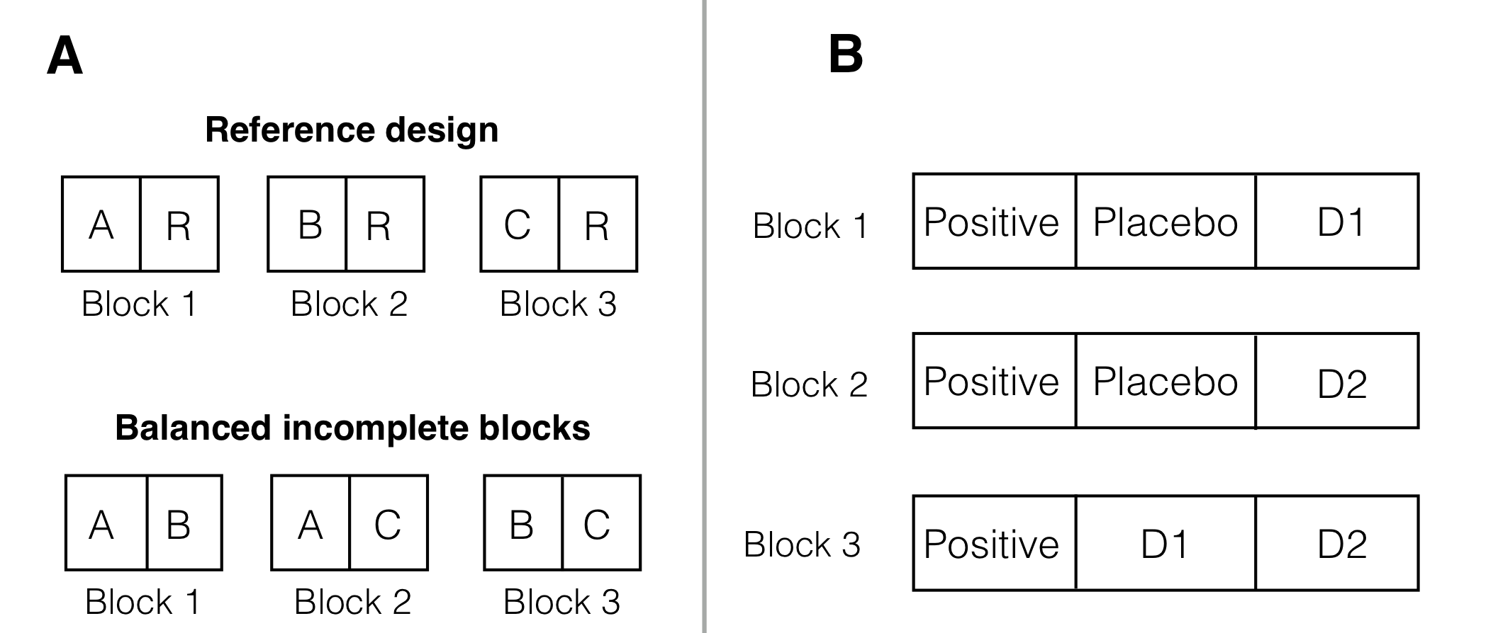
Figure 7.11: A: Reference design for three treatments A,B,C and a reference condition R (top) and BIBD without reference condition (bottom). B: Reference design for three treatments and common positive control as reference condition with block size three.
Another application of reference designs is the screening of several new treatments against a standard treatment. In this case, selected treatments might be compared among each other in a subsequent experiment, and removal of unpromising candidates in the first round might reduce these later efforts.
Generating a simple reference design is straightforward: since each block of size \(s\) contains the reference condition, it has \(s-1\) remaining experimental units for accommodating a subset of the \(k-1\) non-control treatments. This translates into finding a BIBD for \(k-1\) treatments in blocks of size \(s-1\). The main analysis of this design is based on Dunnett-type contrasts, where each treatment level is compared to the reference level. The same considerations as for a CRD with Dunnett-type contrasts then apply, and we might think about using more than one unit per block for the reference condition to improve precision. A balance has then to be struck between improving the comparisons within each block by using more than one replicate of the control condition, and the need to use more blocks and introduce more uncertainty by having smaller block sizes available for the treatment conditions.
For our drug example, we might introduce a positive control condition in addition to the placebo group. A reference design with block size \(s=3\) then requires \(b=3\) blocks, with treatment assignments (positive, placebo, \(D1\)) for the first, (positive, placebo, \(D2\)) for the second, and (positive, \(D1\), \(D2\)) for the third block; this is simply a BIBD with \(s=2\) and \(k=3\), augmented by adding the positive treatment to each block. A single replication is shown in Figure 7.11B.
The same principle extends to constructing reference designs with more than one reference level. In our example, we might want to compare each drug to positive and placebo (negative) control groups, and we accommodate the remaining treatment factor levels in blocks of size \(s-2\). If the available block size is \(s=3\), then no remaining treatment levels co-occur in the same block. Comparisons of these levels to reference levels than profit from blocking, but comparisons between the remaining treatment levels do not.
7.4 Multiple Blocking Factors
7.4.1 Introduction
The unit structure of (G)RCBD and BIBD experimental designs consists of only two unit factors: the blocks and the experimental units nested in blocks. We now discuss unit structures with more than one blocking factor; these can be nested or crossed.
7.4.2 Nesting Blocks
Nesting blocking factors allows us to replicate already blocked designs, to combine several properties for grouping, and to disentangle the variance components of different levels of grouping. It is also sometimes dictated by the logistics of the experiment. We consider only designs with two nested blocking factors, but our discussion directly extends to longer chains of nested factors.
We saw that we can replicate a completely randomized design by crossing its treatment structure with a factor to represent the replication; in our example, we used a CRD with three drugs in two laboratories, each laboratory providing one replicate of the CRD. The same idea allows replicating more complex designs: to replicate our RCBD for drug comparisons blocked by litter in two laboratories, for example, we again cross the treatment structure with a new factor (Lab) with two levels. Since each litter is unique to one laboratory, (Litter) from the original RCBD is nested in (Lab), and both are crossed with Drug, since each drug is assigned to each litter in both laboratories. This yields the treatment and unit structures shown in Figure 7.12A,B. The experiment design in Figure 7.12C has two block-by-treatment interactions, and the three-way interaction is an interaction of a lab-specific litter with the treatment factor. This experiment cannot by analyzed using analysis of variance, because we cannot specify the block-by-treatment interactions; the linear mixed model is y ~ drug + (1|lab/litter) + (1|lab:drug) + (1|lab:litter:drug); note that (1|lab/litter)=(1|lab)+(1|lab:litter).
If we carefully select the blocking factors, we can assume these interactions to be negligible and arrive at the much simpler experiment design in Figure 7.12D. Our experiment again uses 24 mice, with four litters per laboratory, and each litter is a block with one replicate per drug. The model specification is y ~ drug + Error(lab/litter) for an analysis of variance, and y ~ drug + (1|lab/litter) for a linear mixed model. As more than one litter is used per lab, the linear mixed model directly provides us with estimates of the between-lab and the between-litter (within lab) variance components. This gives insight into the sources of variation in this experiment and would allow us, for example, to conclude if the blocking by litter was successful on its own, and how discrepant values for the same drug are between different laboratories. Since the two blocks are nested, the omnibus \(F\)-test and contrasts for Drug are calculated within each litter and then averaged over litters within labs.
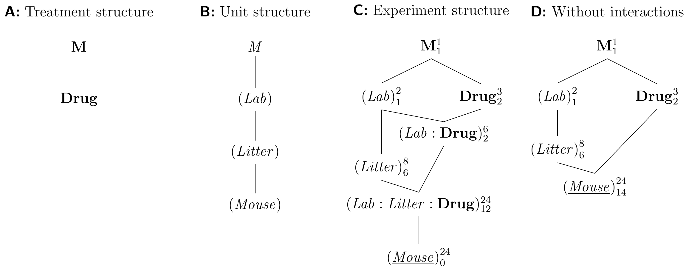
Figure 7.12: Randomized complete block design for determining effect of two different drugs and placebo treatments on enzyme levels in mice, replicated in two laboratories. A: Treatment structure. B: Unit structure with three nested factors. C: Full experiment structure with block-by-treatment interactions. D: Experiment structure if these interactions are negligible.
This type of design can be extended to an arbitrary number of nested blocks and we might use two labs, two cages per lab, and two litters per cage for our example. As long as each nested factor is replicated, we are able to estimate corresponding variance components. If a factor is not replicated (e.g., we use a single litter per lab), then there are no degrees of freedom for the nested blocking factor, and the effects of both blocking factors are completely confounded. Effectively, such a design uses a single blocking factor, where each level is a combination of lab and litter.
We should keep in mind that variance components are harder to estimate than averages, and estimates based on low replication are imprecise. This is not a problem if our goal is removal of variation from treatment contrasts, but sufficient replication is necessary if estimation of variance components is a primary goal of the experiment. Sample size determination for variance component estimation is covered in more specialized texts.
7.4.3 Crossing Blocks: Latin Squares
Nesting blocking factors essentially results in replication of (parts of) the design. In contrast, crossing blocking factors allows us to control several sources of variation simultaneously. The most prominent example is the latin square design, which consists of two crossed blocking factors simultaneously crossed with a treatment factor, such that each treatment level occurs once in each level of the two blocking factors.
For example, we might be concerned about the effect of litters on our drug comparisons, but suspect that the position of the cage in the rack also affects the observations. The latin square design removes both between-litter and between-cage variation from the drug comparisons. For three drugs, this design requires three litters of three mice each, and three cages. Crossing litters and cages results in one mouse per litter in each cage. The drugs are then randomized on the intersection of litters and cages (i.e., on mice) such that each drug occurs once in each cage and once in each litter.
The Hasse diagrams for this design are shown in Figure 7.13. The crucial observation is that none of the potential block-by-block or block-by-treatment interactions can be estimated, since each combination of block levels or block-treatment combinations occurs only once. In particular, the intersection of a cage and a litter is a single mouse, and thus (Cage:Litter) is completely confounded with (Mouse) in this example.
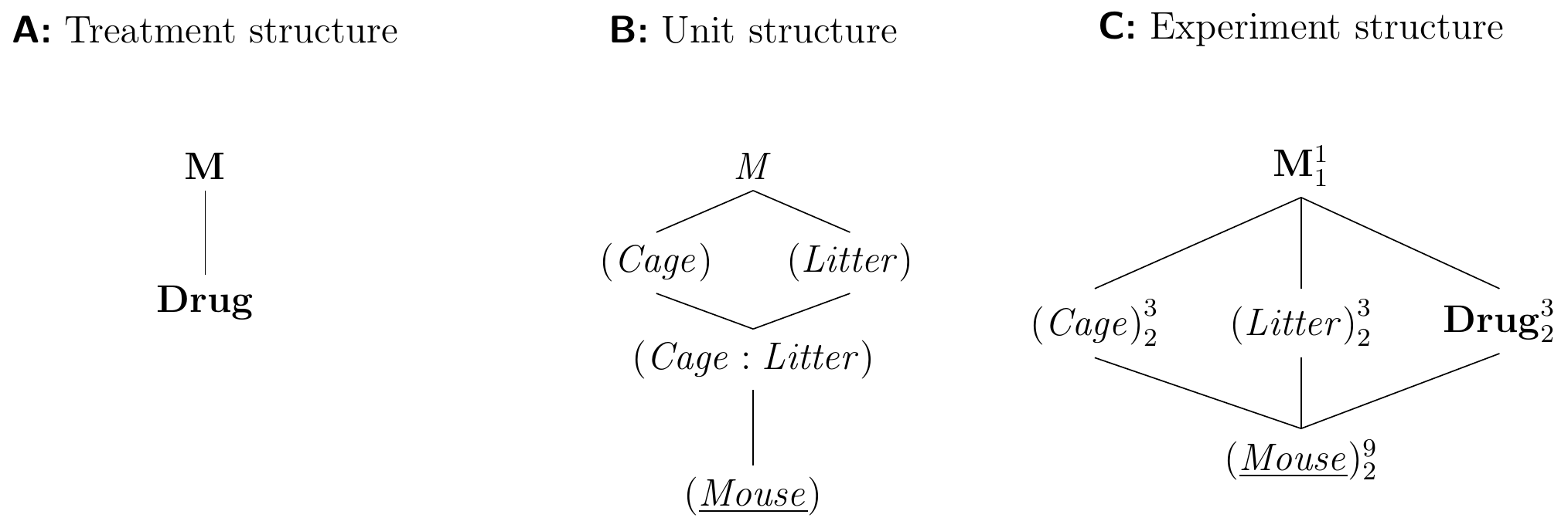
Figure 7.13: Latin square with cage and litter as random row/column effects and three drug treatment levels.
An example layout of this design is shown in Figure 7.14A, where the two blocking factors are given as rows and columns. Each treatment occurs exactly once per row and once per column and the latin square design imposes two simultaneous constraints on the randomization of drugs on mice.
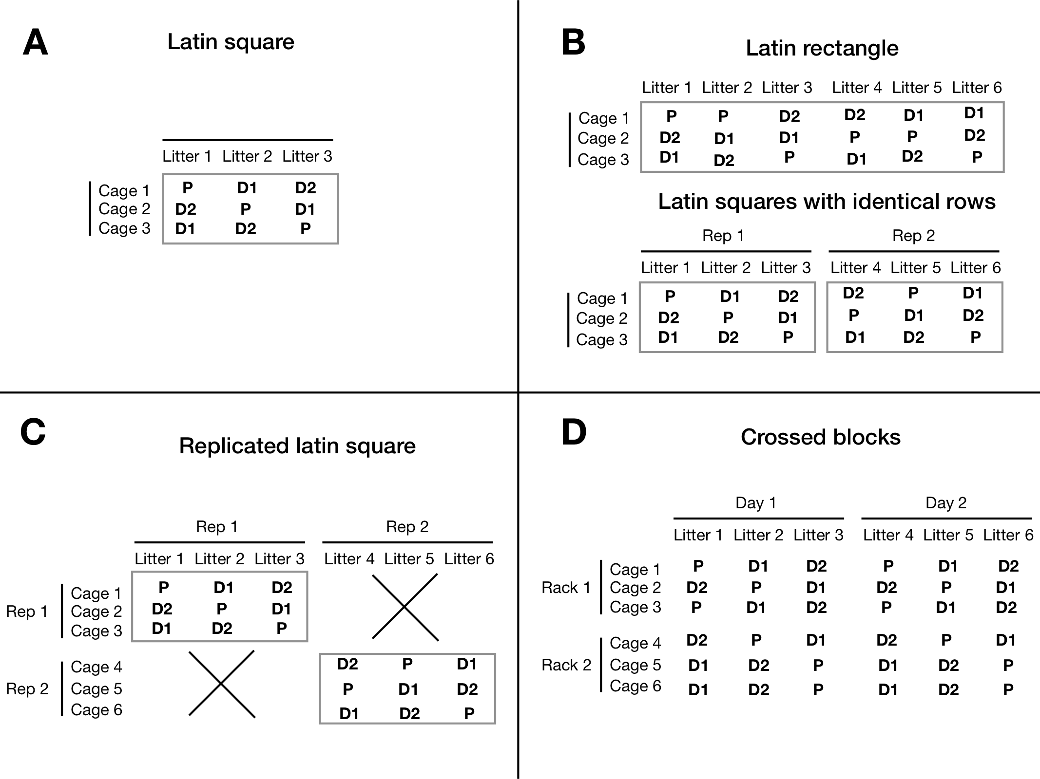
Figure 7.14: A: Latin square using cage and litter and three drug treatments. B: Replication keeping the same cages, and using more litters without (top) and with (bottom) forming latin squares. C: Full replication with new rows and columns. D: Two fully crossed blocks.
With all interactions negligible, data from a latin square design are analyzed by an additive model
\[
y_{ijk} = \mu + \alpha_i + c_j + r_k + e_{ijk}\;,
\]
where \(\mu\) is the grand mean, \(\alpha_i\) the treatment parameters, and \(c_j\) (resp. \(r_k\)) are the random column (resp. row) parameters. This model is again in direct correspondence to the experiment diagram and is specified as y ~ drug + Error(cage+litter), respectively y ~ drug + (1|cage) + (1|litter).
We can interpret the latin square design as a blocked RCBD: ignoring the cage effect, for example, the experiment structure is identical to an RCBD blocked by litter. Conversely, we have an RCBD blocked on cages when ignoring the litter effect. The remaining blocking factor blocks the whole RCBD. The requirement of having each treatment level once per cage and litter implies that the number of cages must equal the number of litters, and that both must also equal the number of treatments. These constraints pose some complications for the randomization of treatment levels to mice, and randomization is usually done by software; many older books on experimental design also contain tables of latin square designs with few treatment levels.
Replicating Latin Squares
A design with a single latin square often lacks sufficient replication: for \(k=2\), \(k=3\), and \(k=4\) treatment levels, we only have \(0\), \(2\), and \(6\) residual degrees of freedom, respectively. We therefore consider several options for generating \(r\) replicates of a latin square design. In each case, the Hasse diagram allows us to calculate the resulting error degrees of freedom and to specify an appropriate linear model.
First, we might consider replicating columns while keeping the rows, using \(rk\) column factor levels instead of \(k\). The same logic applies to keeping columns and replicating rows, of course. The two experiments in Figure 7.14B illustrate this design for a two-fold replication of the \(3\times 3\) latin square, where we use six litters instead of three, but keep using the same three cages in both replicates. In the top part of the panel, we do not impose any new restrictions on the allocation of drugs and only require that each drug occurs the same number of times in each cage, and that each drug is used with each litter. In particular, the first three columns do not form a latin square in themselves. This design is called a , and its experiment structure is shown in Figure 7.15A with model specification y ~ drug + Error(cage+litter) or y ~ drug + (1|cage)+(1|litter).
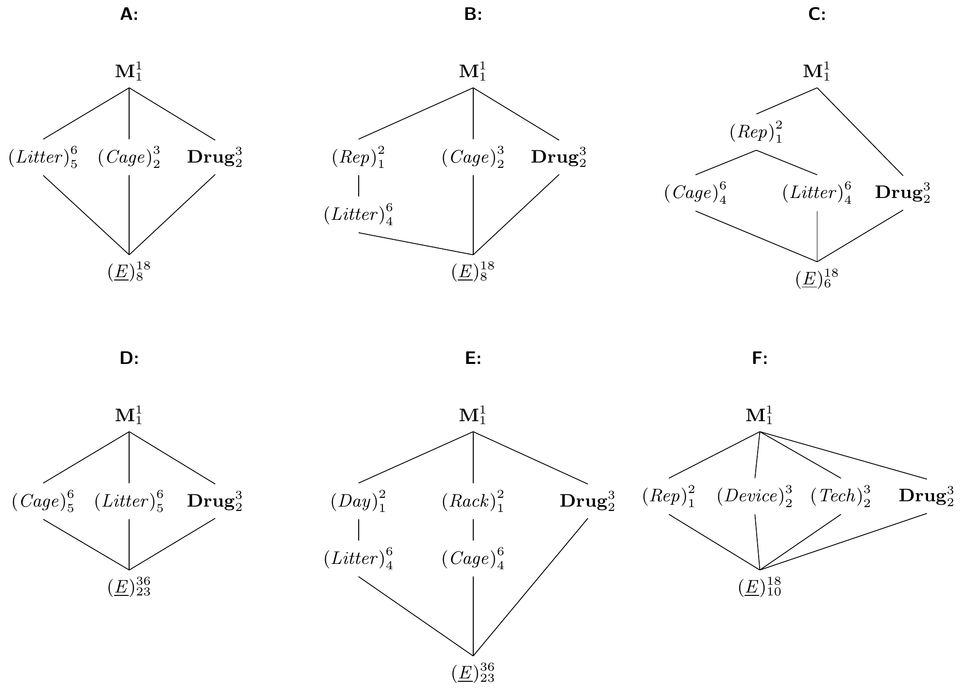
Figure 7.15: Replication of latin square design. A: Latin rectangle with six columns and three rows. B: Two sets of three columns with identical rows. C: New rows and columns in each replicate. D: Fully crossed blocks, not a latin square. E: Keeping both row and column levels with two independently randomized replicates. F: Independent replication of rows and columns.
We can also insist that each replicate forms a proper latin square in itself. That means we organize the columns in two groups of three as shown in the bottom of Figure 7.14B. In the diagram in Figure 7.15B, this is reflected by a new grouping factor (Rep) with two levels, in which the column factor (Litter) is nested. The model is specified as y ~ drug + Error(cage+rep/litter) or y ~ drug + (1|cage)+(1|rep/litter).
By nesting both blocking factors in the replication, we find yet another useful design that uses different row and column factor levels in each replicate of the latin square as shown in Figure 7.14C. The corresponding diagram is Figure 7.15C and yields the model y ~ drug + Error(rep/(cage+litter)) respectively y ~ drug + (1|rep) + (1|rep:cage) + (1|rep:litter).
We can also replicate both rows and columns (potentially with different numbers of replication) without restricting any subset of units to a latin square. The experiment is shown in Figure 7.14D and extends the latin rectangle to rows and columns. Here, none of the replicates alone forms a latin square, but all rows and columns have the same number of units for each treatment level. The diagram is shown in Figure 7.15D with model specification y ~ drug + Error(cage+litter) or y ~ drug + (1|cage)+(1|litter). Using this design but insisting on a latin square in each of the four replicates yields the diagram in Figure 7.15E with model y ~ drug + Error(rack/cage+day/litter) or y ~ drug + (1|rack/cage) + (1|day/litter). Given that we still have 23 residual degrees of freedom, we might also include the three remaining random effects (1|rack:day), (1|rack:litter), and (1|day:cage).
Finally, we might use the same row and column factor levels in each replicate. This is rarely the case for random block factors, but we could use our three drugs with three measurement devices and three laboratory technicians, for example, such that each technician measures one mouse for each treatment in each of the three devices. Essentially, this fully crosses the latin square with a new blocking factor and leads to the model specification y ~ drug + Error(rep+device+tech) or y ~ drug + (1|rep) + (1|device) + (1|tech) for Figure 7.15F.
Power Analysis and Sample size
The determination of sample size and power for a crossed-block design requires no new ideas. The noncentrality parameter \(\lambda\) is again the total sample size times the effect size \(f^2\), and we find the correct degrees of freedom for the residuals from the experiment diagram.
For a single latin square, the sample size is necessarily \(k^2\) and increases to \(r\cdot k^2\) if we use \(r\) replicates. The residual degrees of freedom then depend on the strategy for replication. The residual degrees of freedom and the noncentrality parameter are shown in Table 7.6 for a single latin square and three replication strategies: using the same levels for row and column factors, using the same levels for either row or column factor and new levels for the other, and using new levels for both blocking factors. The numerator degrees of freedom are \(k-1\) in each case.
| Design | NCP \(\lambda\) | \(\text{df}_{\text{res}}\) |
|---|---|---|
| Single latin square | \(\lambda=k^2\cdot f^2\) | \((k-1)(k-2)\) |
| Same rows, same columns | \(\lambda=r\cdot k^2\cdot f^2\) | \((k-1)(r(k-1)-3)\) |
| Same rows, new columns | \(\lambda=r\cdot k^2\cdot f^2\) | \((k-1)(rk-2)\) |
| New rows, new columns | \(\lambda=r\cdot k^2\cdot f^2\) | \((k-1)(r(k-1)-1)\) |
Youden Designs
The latin square design requires identical number of levels for the row and column factors. We can use two blocking factors with a balanced incomplete block design to reduce the required number of levels for one of the two blocking factors. These designs are called Youden squares and only use a fraction of the treatment levels in each column (resp. row) and the full set of treatments in each row (resp. column). The idea was first proposed by Youden for studying inoculation of tobacco plants against the mosaic virus (Youden 1937), and his experiment layout is shown in Figure 7.16.
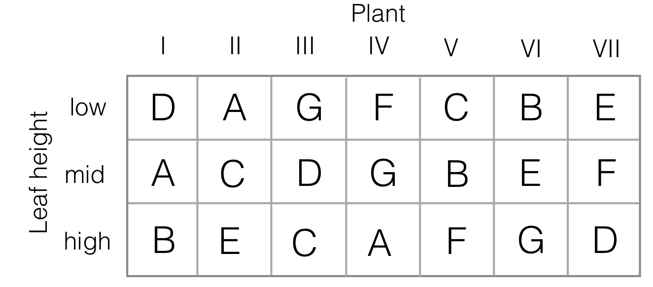
Figure 7.16: Experiment layout for Youden square. Seven plants are considered (I–VII) with seven different inoculation treatments (A–G). In each plant, three leafs at different heights (low/mid/high) are inoculated. Each inoculation occurs once at each height, and the assignment of treatments to plants forms a balanced incomplete block design.
In the experiment, seven plants were considered with seven different inoculation treatments, applied to individual leafs. It was suspected that the height of a plant’s leaf influences the effect of the virus, and leaf height was used as a second blocking factor with three levels (low, middle, high). Crossing the two blocking factors leads to a \(3\times 7\) layout. The treatment levels are randomly allocated such that each treatment occurs once per leaf height (i.e., each inoculation occurs once in each column). The columns form a balanced incomplete block design of \(k=7\) treatments in \(b=7\) blocks of size \(s=3\), leading to \(r=3\) occurrences of each treatment, and \(\lambda=1\) blocks containing each pair of treatments, in accordance with the defining equations (7.3).
7.5 Notes and Summary
Notes
Different ways of replication lead to variants of the GRCBD and are presented in Addelman (1969) and Gates (1995). Variants of blocked designs with different block sizes are discussed in Pearce (1964), and the question of treating blocks as random or fixed in Dixon (2016). Evaluation and testing of blocks is reviewed in Samuels, Casella, and McCabe (1991). Excellent discussions of interactions between different types of factors (e.g., treatment-treatment or treatment-classification) are given in Cox (1984) and de Gonzalez and Cox (2007).
Blocking designs are also important in animal experiments (Lazic and Essioux 2013; Festing 2014), and replicating pre-clinical experiments in at least two laboratories can greatly increase reproducibility (Karp 2018).
The idea of a latin square can be extended to more than two blocking factors; with three factors, such designs are called graeco-latin squares.
Using R
Linear mixed models are covered in R by the lme4 package (Bates et al. 2015) and its lmer() function, which we use exclusively in this book. This package does not provide \(p\)-values, which we can augment by additionally loading the lmerTest package (Kuznetsova, Brockhoff, and Christensen 2017). The linear mixed models are specified similarly to linear models, and random effects are introduced using the (X|G) construct that produces random effects for a factor X grouped by G. We only consider X=1, which produces random intercepts (or offsets) for each level of the factor G. Note that while crossed random factors R and C can be specified in aov() using Error(R+C), the equivalent notation (1|R+C) is not allowed in lmer(), and we use (1|R)+(1|C) instead. A comprehensive textbook on linear mixed models in R is Galecki and Burzykowski (2013); it captures many more uses of these models, such as analysis of longitudinal data.
Latin squares, balanced incomplete block designs and Youden designs are conveniently found and randomized by the functions design.lsd(), design.bib() and design.youden() in the agricolae package. For our example, design.bib(trt=c("Placebo", "D1", "D2"), k=2) yields our first BIBD with \(k=3\) and \(s=2\), and design.youden(trt=LETTERS[1:7], r=3) generates the Youden design of Figure 7.16.
Contrast analysis is based on either aov() or lmer() for estimating the linear model, and estimated marginal means from emmeans(), where results from aov() are based exclusively on the intra-block information and can differ from those based on lmer().
Summary
Crossing a unit factor with the treatment structure leads to a blocked design, where each treatment occurs in each level of the blocking factor. This factor organizes the experimental units into groups, and treatment contrasts can be calculated within each group before averaging over groups. This effectively removes the variation captured by the blocking factor from any treatment comparisons. If experimental units are more similar within the same group than between groups, then this strategy can lead to substantial increase in precision and power, without increasing the sample size. The price we pay is slightly larger organizational effort to create the groups, randomize the treatments independently within each group, and to keep track of which experimental unit belongs to which group for the subsequent analysis.
The most common blocking design is the randomized complete block design, where each treatment occurs once per block. Its analysis requires the assumption of no block-by-treatment interaction, which the experimenter can ensure by suitable choice of the blocking factor. The efficiency of blocking is evaluated by appropriate effect sizes, such as the proportion of variation attributed to the blocking. It typically deteriorates if the block size becomes too large, since experimental units then become more heterogeneous. A balanced incomplete block design allows blocking of simple treatment structures if only a subset of treatments can be accommodated in each block.
Multiple blocking factors can be introduced in the unit structure. Nesting them enables estimation of their respective variance components, while crossing leads to row-column designs that control for two sources of variation simultaneously.
Blocked designs yield ANOVA results with multiple error strata, and only the lowest—within-block—stratum is typically used for analysis. Linear mixed models account for all information, and results might differ slightly from an ANOVA if the design is not fully balanced.