Chapter 4 Comparing More than Two Groups: One-Way ANOVA

4.1 Introduction

We extend our discussion from experiments with two treatment groups to experiments with $k$ treatment groups, assuming completely random treatment allocation. In this chapter, we develop the analysis of variance framework to address the omnibus null hypothesis that all group means are equal and there is no difference between the treatments. The main idea is to partition the overall variation in the data into one part attributable to differences between the treatment group means, and a residual part. We can then test equality of group means by comparing variances between group means and within each group using an $F$-test.

We also look at corresponding effect size measures to quantify the overall difference between treatment group means. The associated power analysis uses the noncentral $F$-distribution, where the noncentrality parameter is the product of experiment size and effect size. Several simplifications allow us to derive a portable power formula for quickly approximating the required sample size.

The analysis of variance is intimately linked to a linear model, and we formally introduce Hasse diagrams to describe the logic of the experiment and to derive the corresponding linear model and its specification in statistical software.

4.2 Experiment and Data

We consider investigating four drugs for their properties to alter the metabolism in mice, and we take the level of a liver enzyme as a biomarker to indicate this alteration, where higher levels are considered as “better.” Metabolization and elimination of the drugs might be affected by the fatty acid metabolism, but for the moment we control this aspect by feeding all mice with the same low fat diet and return to the diet effect in Chapter 6.

Table 4.1: Measured enzyme levels for four drugs assigned to eight mice each.
D1	13.94	16.04	12.70	13.98	14.31	14.71	16.36	12.58
D2	13.56	10.88	14.75	13.05	11.53	13.22	11.52	13.99
D3	10.57	8.40	7.64	8.97	9.38	9.13	9.81	10.02
D4	10.78	10.06	9.29	9.36	9.04	9.41	6.86	9.89

The data in Table 4.1 and Figure 4.1A show the observed enzyme levels for $N=n\cdot k=$ 32 mice, with $n=$ 8 mice randomly assigned to one of the $k=4$ drugs $D1$, $D2$, $D3$, and $D4$. We denote the four average treatment group responses as $\mu_1,\dots,\mu_4$; we are interested in testing the omnibus hypothesis $H_0: \mu_1=\mu_2=\mu_3=\mu_4$ that the group averages are identical and the four drugs therefore all have the same effect on the enzyme levels.

Other interesting questions regard estimation and testing of specific treatment group comparisons, which we postpone to Chapter 5.

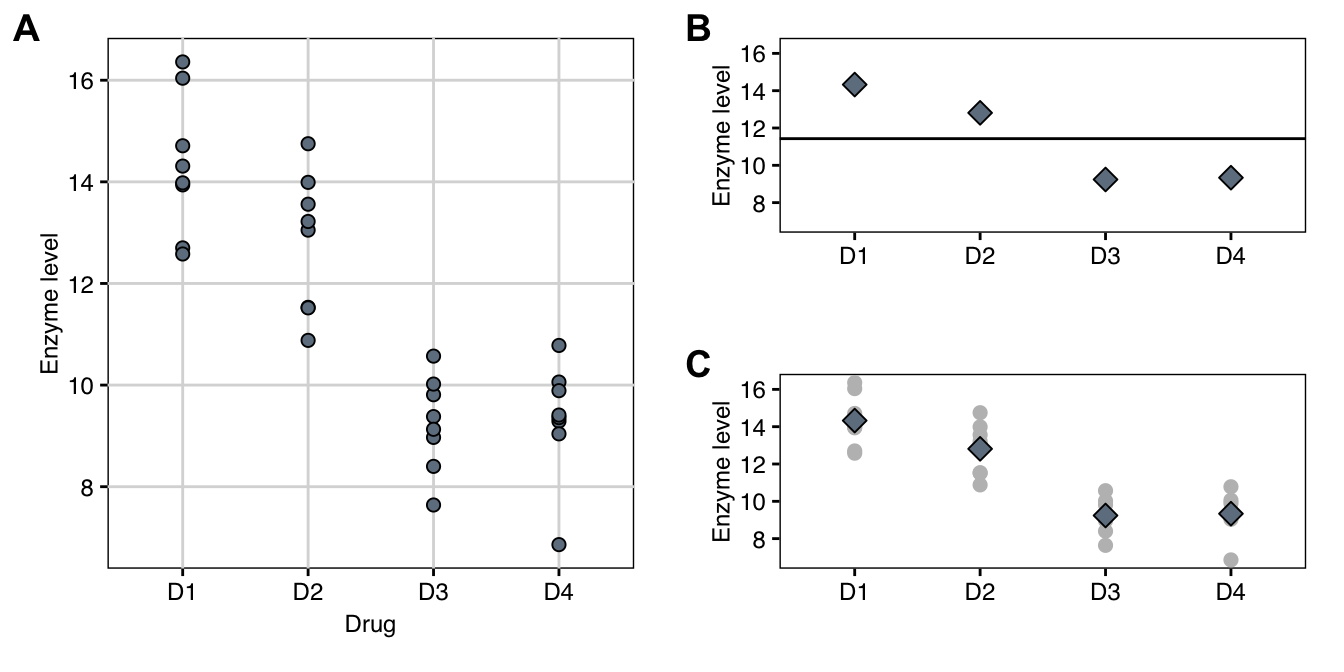
Observed enzyme levels in response to four drug treatments with eight mice per treatment group. A: Individual observations by treatment group. B: Grand mean (horizontal line) and group means (diamonds) used in estimating the between-group variance. C: Individual responses (grey points) are compared to group means (black diamonds) for estimating the within-group variance.

Figure 4.1: Observed enzyme levels in response to four drug treatments with eight mice per treatment group. A: Individual observations by treatment group. B: Grand mean (horizontal line) and group means (diamonds) used in estimating the between-group variance. C: Individual responses (grey points) are compared to group means (black diamonds) for estimating the within-group variance.

4.3 One-Way Analysis of Variance

In a balanced completely randomized design, we randomly allocate $k$ treatments on $N=n\cdot k$ experimental units. We assume that the response $y_{ij}\sim N(\mu_i,\sigma_e^2)$ of the $j$th experimental unit in the $i$th treatment group is normally distributed with group-specific expectation $\mu_i$ and common variance $\sigma_e^2$, with $i=1\dots k$ and $j=1\dots n$; each group then has $n$ experimental units.

4.3.1 Testing Equality of Means by Comparing Variances

For $k=2$ treatment groups, the omnibus null hypothesis is $H_0: \mu_1=\mu_2$ and can be tested using a $t$-test on the group difference $\Delta=\mu_1-\mu_2$. For $k>2$ treatment groups, the corresponding omnibus null hypothesis is $H_0:\mu_1=\dots =\mu_k$, and the idea of using a single difference for testing does not work.

The crucial observation for deriving a test statistic for the general omnibus null hypothesis comes from changing our perspective on the problem: if the treatment group means $\mu_i\equiv \mu$ are all equal, then we can consider their estimates $\hat{\mu}_i=\sum_{j=1}^n y_{ij}/n$ as independent ‘samples’ from a normal distribution with mean $\mu$ and variance $\sigma_e^2/n$ (Figure 4.1B). We can then estimate their variance using the usual formula \[ \widehat{\text{Var}}(\hat{\mu}_i) = \sum_{i=1}^k (\hat{\mu}_i-\hat{\mu})^2/(k-1)\;, \] where $\hat{\mu}=\sum_{i=1}^k \hat{\mu}_i/k$ is an estimate of the grand mean $\mu$. Since $\text{Var}(\hat{\mu}_i)=\sigma_e^2/n$, this provides us with an estimator \[ \tilde{\sigma}_e^2=n\cdot\widehat{\text{Var}}(\hat{\mu}_i)=n\cdot\sum_{i=1}^k (\hat{\mu}_i-\hat{\mu})^2/(k-1) \] for the variance $\sigma_e^2$ that only considers the dispersion of group means around the grand mean and is independent of the dispersion of individual observations around their group mean.

On the other hand, our previous estimator pooled over groups is \[ \hat{\sigma}_e^2 = \left( \underbrace{ \frac{\sum_{j=1}^n(y_{1j}-\hat{\mu}_1)^2}{n-1} }_{ \text{variance group $1$} } +\cdots+ \underbrace{ \frac{\sum_{j=1}^n(y_{kj}-\hat{\mu}_k)^2}{n-1} }_{ \text{variance group $k$} } \right)/k = \sum_{i=1}^k\sum_{j=1}^n \frac{(y_{ij}-\hat{\mu}_i)^2}{N-k} \] and also estimates the variance $\sigma_e^2$ (Figure 4.1C). It only considers the dispersion of observations around their group means, and is independent of the $\mu_i$ being equal. For example, we could add a fixed number to all measurements in one group and this would affect $\tilde{\sigma}_e^2$ but not $\hat{\sigma}_e^2$.

The two estimators have expectations \[ \mathbb{E}(\tilde{\sigma}_e^2) = \sigma_e^2 + \underbrace{\frac{1}{k-1}\,\sum_{i=1}^k n\cdot(\mu_i-\mu)^2}_{Q} \quad\text{and}\quad \mathbb{E}(\hat{\sigma}_e^2) = \sigma_e^2\;, \] respectively. Thus, while $\hat{\sigma}_e^2$ is always an unbiased estimator of the residual variance, the estimator $\tilde{\sigma}_e^2$ has bias $Q$—the between-groups variance—but is unbiased precisely if $H_0$ is true and $Q=0$. If $H_0$ is true, then the ratio \[ F = \frac{\tilde{\sigma}_e^2}{\hat{\sigma}_e^2} \sim F_{k-1,N-k} \] has an $F$-distribution with $k-1$ numerator and $N-k$ denominator degrees of freedom. The distribution of $F$ deviates more from this distribution the larger the term $Q$ becomes and the ‘further away’ the observed group means are from equality. The corresponding $F$-test thus provides the required test of the omnibus hypothesis $H_0:\mu_1=\cdots =\mu_k$.

For our example, we estimate the four group means $\hat{\mu}_1=$ 14.33, $\hat{\mu}_2=$ 12.81, $\hat{\mu}_3=$ 9.24, and $\hat{\mu}_4=$ 9.34 and a grand mean $\hat{\mu}=$ 11.43. Their squared differences are $(\hat{\mu}_1-\hat{\mu})^2=$ 8.42, $(\hat{\mu}_2-\hat{\mu})^2=$ 1.91, $(\hat{\mu}_3-\hat{\mu})^2=$ 4.79, and $(\hat{\mu}_4-\hat{\mu})^2=$ 4.36. With $n=$ 8 mice per treatment group, this gives the two estimates $\tilde{\sigma}_e^2=$ 51.96 and $\hat{\sigma}_e^2=$ 1.48 for the variance. Their ratio is $F=$ 35.17 and comparing it to an $F$-distribution with $k-1=$ 3 numerator and $N-k=$ 28 denominator degrees of freedom gives a $p$-value of $p=$ 1.24$\times 10^{-9}$, indicating strongly that the group means are not identical.

Perhaps surprisingly, the $F$-test is identical to the $t$-test for $k=2$ treatment groups, and will give the same $p$-value. We can see this directly using a little algebra (note $\hat{\mu}=(\hat{\mu}_1+\hat{\mu}_2)/2$ and $N=2\cdot n$): \[ F = \frac{n\cdot((\hat{\mu}_1-\hat{\mu})^2+(\hat{\mu}_2-\hat{\mu})^2)/1}{\hat{\sigma}_e^2} = \frac{\frac{n}{2}\cdot \left(\hat{\mu}_1-\hat{\mu}_2\right)^2}{\hat{\sigma}_e^2} = \left(\frac{\hat{\mu}_1-\hat{\mu}_2}{\sqrt{2}\hat{\sigma}_e/\sqrt{n}}\right)^2=T^2\;, \] and $F_{1,2n-2}=t^2_{2n-2}$. While the $t$-test uses a difference in means, the $F$-test uses the average squared difference from group means to general mean; for two groups, these concepts are equivalent.

4.3.2 Analysis of Variance

Our derivation of the omnibus $F$-test used the decomposition of the data into a between-groups and a within-groups component. We can exploit this decomposition further in the (one-way) analysis of variance (ANOVA) by directly partitioning the overall variation in the data via sums of squares and their associated degrees of freedom. In the words of its originator:

The analysis of variance is not a mathematical theorem, but rather a convenient method of arranging the arithmetic. (Fisher 1934)

The arithmetic advantages of the analysis of variance are no longer relevant today, but the decomposition of the data into various parts for explaining the observed variation remains an easily interpretable summary of the experimental results.

Partitioning the Data

To stress that ANOVA decomposes the variation in the data, we first write each datum $y_{ij}$ as a sum of three components: the grand mean, deviation of group mean to grand mean, and deviation of datum to group mean: \[ y_{ij} = \bar{y}_{\bigcdot\bigcdot} + (\bar{y}_{i\bigcdot}-\bar{y}_{\bigcdot\bigcdot}) + (y_{ij}-\bar{y}_{i\bigcdot})\;, \] where $\bar{y}_{i\bigcdot}=\sum_j y_{ij}/n$ is the average of group $i$, and $\bar{y}_{\bigcdot\bigcdot}=\sum_i\sum_j y_{ij}/nk$ is the grand mean, and a dot indicates summation over the corresponding index.

For example, the first datum in the second group, $y_{21}=$ 13.56, is decomposed into the grand mean $\bar{y}_{\bigcdot\bigcdot}=$ 11.43, the deviation from group mean $\bar{y}_{2\bigcdot}=$ 12.81 to grand mean $(\bar{y}_{2\bigcdot}-\bar{y}_{\bigcdot\bigcdot})=$ 1.38 and the residual $y_{21}-\bar{y}_{2\bigcdot}=$ 0.75.

Sums of Squares

We quantify the overall variation in the observations by the total sum of squares, the summed squared distances of each datum $y_{ij}$ to the estimated grand mean $\bar{y}_{\bigcdot\bigcdot}$.

Following the partition of each datum, the total sum of squares also partitions into two parts: (i) the treatment (or between-groups) sum of squares which measures the variation between group means and captures the variation explained by the systematic differences between the treatments, and (ii) the residual (or within-groups) sum of squares which measures the variation of responses within each group and thus captures the unexplained random variation: \[ \text{SS}_\text{tot} = \sum_{i=1}^k\sum_{j=1}^{n}(y_{ij}-\bar{y}_{\bigcdot\bigcdot})^2 = \underbrace{\sum_{i=1}^k n\cdot (\bar{y}_{i\bigcdot}-\bar{y}_{\bigcdot\bigcdot})^2}_{\text{SS}_\text{trt}} + \underbrace{\sum_{i=1}^k\sum_{j=1}^{n} (y_{ij}-\bar{y}_{i\bigcdot})^2}_{\text{SS}_\text{res}} \;, \] The intermediate term $2\sum_{i}\sum_{j} (y_{ij}-\bar{y}_{i\bigcdot})(\bar{y}_{i\bigcdot}-\bar{y}_{\bigcdot\bigcdot})=0$ vanishes because $\text{SS}_\text{trt}$ is based on group means and grand mean, while $\text{SS}_\text{res}$ is independently based on observations and group means; the two are orthogonal.

For our example, we find a total sum of squares of $\text{SS}_\text{tot}=$ 197.26, a treatment sum of squares $\text{SS}_\text{trt}=$ 155.89, and a residual sum of squares $\text{SS}_\text{res}=$ 41.37; as expected the latter two add precisely to $\text{SS}_\text{tot}$. Thus, most of the observed variation in the data is due to systematic differences between the treatment groups.

Degrees of Freedom

Associated with each sum of squares term are its degrees of freedom, the number of independent components used to calculate it.

The total degrees of freedom for $\text{SS}_{\text{tot}}$ are $\text{df}_\text{tot}=N-1$, because we have $N$ response values, and need to compute a single value $\bar{y}_{\bigcdot\bigcdot}$ to find the sum of squares.

The treatment degrees of freedom are $\text{df}_\text{trt}=k-1$, because there are $k$ treatment means, estimated by $\bar{y}_{i\bigcdot}$, but the calculation of the sum of squares requires the overall average $\bar{y}_{\bigcdot\bigcdot}$.

Finally, there are $N$ residuals, but we used up 1 degree of freedom for the overall average, and $k-1$ for the group averages, leaving us with $\text{df}_\text{res}=N-k$ degrees of freedom.

The degrees of freedom then decompose as \[ \text{df}_\text{tot} = \text{df}_\text{trt} + \text{df}_\text{res} \;. \] This decomposition tells us how much of the data we ‘use up’ for calculating each sum of squares component.

Mean Squares

Dividing a sum of squares by its degrees of freedom gives the corresponding mean squares, which are exactly our two variance estimates. The treatment mean squares are given by \[ \text{MS}_\text{trt} = \frac{\text{SS}_\text{trt}}{\text{df}_\text{trt}} = \frac{\text{SS}_\text{trt}}{k-1} = \tilde{\sigma}_e^2 \;, \] and are our first variance estimate based on group means and grand mean, while the residual mean squares \[ \text{MS}_\text{res} = \frac{\text{SS}_\text{res}}{\text{df}_\text{res}} = \frac{\text{SS}_\text{res}}{N-k} = \hat{\sigma}_e^2\;, \] are our second independent estimator for the within-group variance. We find $\text{MS}_\text{res}=$ 41.37 / 28 = 1.48 and $\text{MS}_\text{trt}=$ 155.89 / 3 = 51.96 for our example.

In contrast to the sum of squares, the mean squares do not decompose by factor and $\text{MS}_\text{tot}=\text{SS}_\text{tot}/(N-1)=$ 6.36 $\not=\text{MS}_\text{trt}+\text{MS}_\text{res}=$ 53.44.

Omnibus $F$-test

Our $F$-statistic for testing the omnibus hypothesis $H_0:\mu_1=\cdots=\mu_k$ is then \[ F = \frac{\text{MS}_\text{trt}}{\text{MS}_\text{res}} = \frac{\text{SS}_\text{trt}/\text{df}_\text{trt}}{\text{SS}_\text{res}/\text{df}_\text{res}} \sim F_{\text{df}_\text{trt}, \text{df}_\text{res}}\;, \] and we reject $H_0$ if the observed $F$-statistic exceeds the $(1-\alpha)$-quantile $F_{1-\alpha,\text{df}_\text{trt}, \text{df}_\text{res}}$.

Based on the sum of squares and degrees of freedom decompositions, we again find the observed test statistic of $F=$ 51.96 / 1.48 = 35.17 on $\text{df}_\text{trt}=$ 3 and $\text{df}_\text{res}=$ 28 degrees of freedom, corresponding to a $p$-value of $p=$ 1.24$\times 10^{-9}$.

ANOVA Table

The results of an ANOVA are usually presented in an ANOVA-table such as Table 4.2 for our example.

Table 4.2: Manually calculated summary table for analysis of variance.
Source	df	SS	MS	F	p
drug	3	155.89	51.96	35.2	1.24e-09
residual	28	41.37	1.48

An ANOVA table has one row for each source of variation, and the first column gives the name of each source. The remaining columns give (i) the degrees of freedom available for calculating the sum of squares (indicating how much of the data is ‘used’ for this source of variation); (ii) the sum of squares to quantify the variation attributed to the source; (iii) the resulting mean squares used for testing; (iv) the observed value of the $F$-statistic for the omnibus null hypothesis and (v) the corresponding $p$-value.

4.3.3 Effect Size Measures

The raw difference $\Delta$ or the standardized difference $d$ provide easily interpretable effect size measures for the case of $k=2$ treatment groups that we can use in conjunction with the $t$-test. We now introduce three effect size measures for the case of $k>2$ treatment groups for use in conjunction with an omnibus $F$-test.

A simple effect size measure is the variation explained, which is the proportion of the factor’s sum of squares of the total sum of squares: \[ \eta^2_\text{trt} = \frac{\text{SS}_\text{trt}}{\text{SS}_\text{tot}} = \frac{\text{SS}_\text{trt}}{\text{SS}_\text{trt} + \text{SS}_\text{res}}\;. \] A large value of $\eta^2_\text{trt}$ indicates that the majority of the variation is not due to random variation between observations in the same treatment group, but rather due to the fact that the average responses to the treatments are different. In our example, we find $\eta^2_\text{trt}=$ 155.89 $/$ 197.26 $=$ 0.79, confirming that the differences between drugs are responsible for 79% of the variation in the data.

The raw effect size measures the average deviation between group means and the grand mean: \[ b^2=\frac{1}{k}\sum_{i=1}^k(\mu_i-\mu)^2=\frac{1}{k}\sum_{i=1}^k\alpha_i^2\;. \] A corresponding standardized effect size was proposed in Cohen (1992): \[ f^2 = b^2/\sigma_e^2 = \frac{1}{k\sigma_e^2}\sum_{i=1}^k \alpha_i^2\;. \] and measures the average deviation between group means and grand mean in units of residual variance. It specializes to $f=d/2$ for $k=2$ groups.

Extending from his classification of effect sizes $d$, Cohen proposed that values of $f>0.1$, $f>0.25$, and $f>0.4$ may be interpreted as small, medium, and large effects (Cohen 1992). An unbiased estimate of $f^2$ is \[ \hat{f}^2 = \frac{\text{SS}_\text{trt}}{\text{SS}_\text{res}} = \frac{k-1}{N-k}\cdot F = \frac{N}{N-k}\cdot\frac{1}{k\cdot\hat{\sigma}_e^2}\sum_{i=1}^k \hat{\alpha}_i^2 \;, \] where $F$ is the observed value of the $F$-statistic, yielding $\hat{f}^2=$ 3.77 for our example; the factor $N/(N-k)$ removes the bias.

The two effect sizes $f^2$ and $\eta^2_\text{trt}$ are translated into each other via \[\begin{equation} f^2 = \frac{\eta^2_\text{trt}}{1-\eta^2_\text{trt}} \quad\text{and}\quad \eta^2_\text{trt} = \frac{f^2}{1+f^2}\;. \tag{4.1} \end{equation}\] Much like the omnibus $F$-test, all three effect sizes quantify any pattern of group mean differences, and do not distinguish if each group deviates slightly from the grand mean, or if one group deviates by a substantial amount while the remaining do not.

4.4 Power Analysis and Sample Size for Omnibus $F$-test

We are often interested in determining the necessary sample size such that the omnibus $F$-test reaches a desired power for a given significance level. Just as before, we need four out of the following five quantities for a power analysis: the two error probabilities $\alpha$ and $\beta$, the residual variance $\sigma_e^2$, the sample size per group $n$ (we only consider balanced designs), and a measure of the minimal relevant effect size (raw or standardized).

4.4.1 General Idea

Recall that under the null hypothesis of equal treatment group means, the deviations $\alpha_i=\mu_i-\mu$ are all zero, and $F=\text{MS}_\text{trt}/\text{MS}_\text{res}$ follows an $F$-distribution with $k-1$ numerator and $N-k$ denominator degrees of freedom.

If the treatment effects are not zero, then the test statistic follows a noncentral $F$-distribution $F_{k-1, N-k}(\lambda)$ with noncentrality parameter \[ \lambda = n\cdot k\cdot f^2 = \frac{n\cdot k\cdot b^2}{\sigma_e^2}= \frac{n}{\sigma_e^2}\cdot \sum_{i=1}^k \alpha_i^2\;. \] The noncentrality parameter is thus the product of the overall sample size $N=n\cdot k$ and the standardized effect size $f^2$ (which can be translated from and to $\eta^2_\text{trt}$ via Eq. (4.1)). For $k=2$, this reduces to the previous case since $f^2=d^2/4$ and $t^2_n(\eta)=F_{1,n}(\lambda=\eta^2)$.

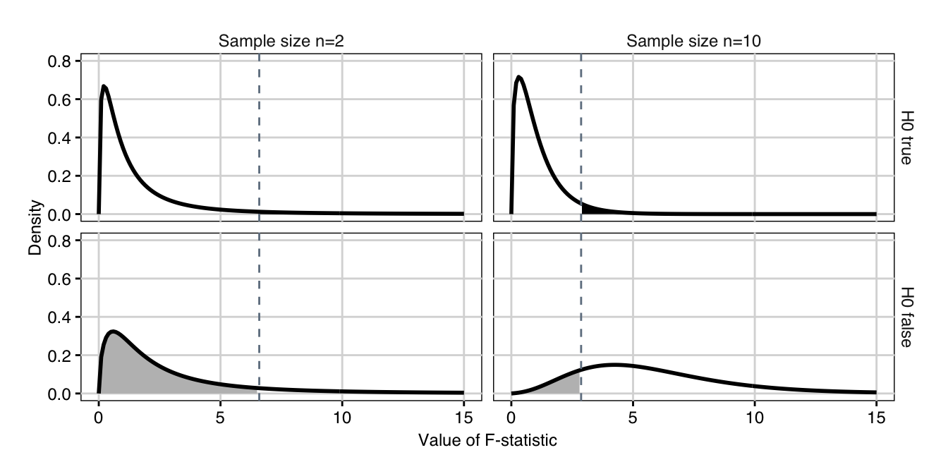
$Distribution of $F$-statistic if $H_0$ is true (top) with false positives (black shaded area), respectively if $H_0$ is false and the first two groups differ by a value of two (bottom) with false negatives (grey shaded area). The dashed line indicates the 95\%-quantile of the central $F$-distribution. Left: sample size n=2; right: sample size n=10.$

Figure 4.2: Distribution of $F$-statistic if $H_0$ is true (top) with false positives (black shaded area), respectively if $H_0$ is false and the first two groups differ by a value of two (bottom) with false negatives (grey shaded area). The dashed line indicates the 95%-quantile of the central $F$-distribution. Left: sample size n=2; right: sample size n=10.

The idea behind the power analysis is the same as for the $t$-test. If the omnibus hypothesis $H_0$ is true, then the $F$-statistic follows a central $F$-distribution with $k-1$ and $N-k$ degrees of freedom, shown in Figure 4.2 (top) for two sample sizes $n=$ 2 (left) and $n=$ 10 (right). The hypothesis is rejected at the significance level $\alpha=5\%$ (black shaded area) whenever the observed $F$-statistic is larger than the 95%-quantile $F_{1-\alpha,\, k-1,\, N-k}$ (dashed line).

If $H_0$ is false, then the $F$-statistic follows a noncentral $F$-distribution. Two corresponding examples are shown in Figure 4.2 (bottom) for an effect size $f^2=$ 0.34 corresponding, e.g., to a difference of $\delta=2$ between first and second treatment group, with no difference between the remaining two treatment groups. We observe that this distribution shifts to higher values with increasing sample size, since its noncentrality parameter $\lambda=n\cdot k\cdot f^2$ increases with $n$. For $n=$ 2, we have $\lambda=2\cdot 4\cdot f^2=$ 2.72 in our example, while for $n=$ 10, we already have $\lambda=10\cdot 4\cdot f^2=$ 13.6. In each case, the probability $\beta$ of falsely not rejecting $H_0$ (a false positive) is the grey shaded area under the density up to the rejection quantile $F_{1-\alpha,\, k-1,\, N-k}$ of the central $F$-distribution. For $n=$ 2, the corresponding power is then $1-\beta=$ 13% which increases to $1-\beta=$ 85% for $n=$ 10.

4.4.2 Defining the Minimal Effect Size

The number of treatments $k$ is usually predetermined, and we then exploit the relation between noncentrality parameter, effect size, and sample size for the power analysis. A main challenge in practice is to decide upon a reasonable minimal effect size $f_0^2$ or $b_0^2$ that we want to reliably detect. Using a minimal raw effect size also requires an estimate of the residual variance $\sigma_e^2$ from previous data or a dedicated preliminary experiment.

A simple method to provide a minimal effect size uses the fact that $f^2\geq d^2/2k$ for the standardized effect size $d$ between any pair of group means. The standardized difference $d_0=\delta_0/\sigma=(\mu_{\text{max}}-\mu_\text{min})/\sigma$ between the largest and smallest group means therefore provides a conservative minimal effect size $f^2_0=d_0^2/2k$ (Kastenbaum, Hoel, and Bowman 1970).

We can improve on the inequality for specific cases, and Cohen proposed three patterns with minimal, medium, and maximal variability of treatment group differences $\alpha_i$, and provided their relation to the minimal standardized difference $d_0$ (Cohen 1988, 276ff).

If only two groups show a deviation from the common mean, we have $\alpha_{\text{max}}=+\delta_0/2$ and $\alpha_{\text{min}}=-\delta_0/2$ for these two groups, respectively, while $\alpha_i=0$ for the $k-2$ remaining groups. Then, $f_0^2=d_0^2/2k$ and our conservative effect size is in fact exact.
If the groups means $\mu_i$ are equally spaced with distances $\delta_0/(k-1)$, then the omnibus effect size is $f_0^2=d_0^2/4\cdot(k+1)/3(k-1)$. For $k=4$ and $d=3$, an example is $\mu_1=1$, $\mu_2=2$, $\mu_3=3$, and $\mu_4=4$.
If half of the groups is at one extreme $\alpha_{\text{max}}=+\delta_0/2$ while the other half is at the other extreme $\alpha_{\text{min}}=-\delta_0/2$, then $f_0^2=d_0^2/4$ if $k$ is even and $f_0^2=d_0^2/4\cdot (1-1/k^2)$ if $k$ is odd. Again for $k=4$ and $d=3$, an example is $\alpha_1=\alpha_3=-1.5$, $\alpha_2=\alpha_4=+1.5$. For $\mu=10$ and $\sigma^2=1$, this corresponds to $\mu_1=\mu_3=8.5$ and $\mu_2=\mu_4=11.5$.

4.4.3 Calculating Power

A simple power analysis function for R is given in Section 4.7 for illustration, while the more flexible built-in procedure power.anova.test() directly provides the necessary calculations. This procedure accepts the number of groups $k$ (groups=), the per-group sample size $n$ (n=), the residual variance $\sigma_e^2$ (within.var=), the power $1-\beta$ (power=), the significance level $\alpha$ (sig.level=), and a modified version of the raw effect size $\nu^2=\sum_i \alpha_i^2/(k-1)$ (between.var=) as its arguments. Given any four of these parameters, it will calculate the remaining one.

We look at a range of examples to illustrate the use of power analysis in R. We assume that our previous analysis was completed and we intend to explore new experiments of the same type. This allows us to use the variance estimate $\hat{\sigma}_e^2$ as our assumed within-group variance for the power analyses, where we round this estimate to $\hat{\sigma}_e^2=$ 1.5 for the following calculations. In all examples, we set our false positive probability to the customary $\alpha=5\%$.

Raw Effect Size $b^2$

From a minimal raw effect size $b_0^2$, we find the corresponding between.var argument as \[ \nu^2_0 = \frac{k}{k-1}\cdot b_0^2\;. \] For example, we might consider an effect with $\alpha_1=\alpha_2=+1$ and $\alpha_3=\alpha_2=-1$, such that $D1$ and $D2$ yield identically higher average enzyme levels, while $D3$ and $D4$ yield correspondingly lower enzyme levels. Then our raw effect size is $b_0^2=((+1)^2+(+1)^2+(-1)^2+(-1)^2)/4=1$ and we use between.var= 1.33 and within.var= 1.5 for our calculation. For a required power of 80%, this yields $n=$ 5 mice per group. Using only $n=$ 2 mice per group, we achieve a power of $1-\beta=$ 21%.

Standardized Effect Size $f^2$

From a minimal standardized effect size $f^2_0$, we find the corresponding between.var argument as \[ \nu^2_0 = \frac{k}{k-1}\cdot\sigma_e^2\cdot f_0^2\;, \] but this formula defeats the purpose of a standardized effect size, since it explicitly requires the residual variance. The solution to this problem comes from noticing that since we measure effects in units of standard deviation, we can set $\sigma_e^2=1$ in this formula and use it in conjunction with within.var=1 to achieve the desired result.

The standardized effect sizes of $f^2_0=$ 0.01 (small), $f^2_0=$ 0.06 (medium), and $f^2_0=$ 0.16 (large) then translate to $\nu_0^2=$ 0.01, $\nu_0^2=$ 0.08, and $\nu_0^2=$ 0.21, respectively.

For a sample size of 10 mice per drug, these minimal effect sizes correspond to a power of 7%, 21%, and 50%, respectively, and to achieve a desired power of 80% would require 274, 45, and 18 mice per drug, respectively.

Range of Group Mean Differences

For finding the required sample size based on a minimal group difference, we plan a follow-up experiment to detect a difference of at least $\delta_0=$ 1 between the average enzyme levels of $D1$ and $D2$. With our assumed variance of $\sigma_e^2=$ 1.5, this corresponds to a standardized effect size of $d_0=\delta_0/\sigma=$ 0.82.

We use Cohen’s first pattern and set $\alpha_1=\delta_0/2$, $\alpha_2=-\delta_0/2$, $\alpha_3=\alpha_4=0$, which yields a standardized effect size of $f^2=$ 0.083, respectively $\eta^2=$ 0.077. Using the formulas above, this corresponds to a between.var parameter of $\nu_0^2=$ 0.17.

The required sample size for a power of 80% is 34 mice per group.

Variance Explained $\eta^2$

To plan an experiment that yields $\eta^2_\text{0,drug}=$ 20% of the variation explained by the differences in drugs, we proceed as for $f_0^2$ and translate this effect size into the between.var argument by \[ \nu_0^2 = \frac{k}{k-1}\cdot \frac{\eta^2_\text{0,drug}}{1-\eta^2_\text{0,drug}}\;, \] using $\sigma_e^2=1$ here and as our within.var argument.

For $k=$ 4 groups, this yields a parameter of $\nu_0^2=$ 0.13 and we can detect this effect size with power $1-\beta=$ 44% for a sample size of $n=$ 10 per treatment group. Similarly, we require $n=$ 20 mice per drug treatment to achieve a desired power of 80%.

Minimal Detectable Effect Size

We can also find the minimal effect size detectable for a given sample size and power. For example, we might plan a similar experiment with the same four drugs, but we have only maximally 20 mice per drug available. Plugging everything in, we find a detectable between-groups variation of $\nu_0^2=$ 0.29, corresponding to an effect size of $f^2=$ 0.14 or $\eta^2_{\text{drug}}=$ 13%.

4.4.4 Power Analysis in Practice

The power calculations for the omnibus $F$-test rely on the same assumptions as the test itself, and require identical residual variances for each treatment group and normally distributed residuals. Results are only marginally affected by moderately different group variances or moderate deviations from normality, but the seemingly precise six decimals of the built-in power.anova.test() should not be taken too literally. More severe errors result if observations are not independent, for example if correlations arise by measuring the same unit multiple times.

Even if all assumptions are matched perfectly, the calculated sample size is still based on an educated guess or a previous estimate of the residual variance. We should therefore make an allowance for a margin of error in our calculations.

We can again use a conservative approach and base our power calculations on the upper confidence limit rather than the variance estimate itself. For our example, the residual variance is $\hat{\sigma}_e^2\approx$ 1.5 with a 95%-confidence interval of [0.94, 2.74]. For $k=$ 4 groups, a desired power of 80% and a significance level of 5%, detecting a raw effect of $b_0^2=$ 0.12 ($f_0^2=$ 0.08) requires 34 mice per group. Taking the upper confidence limit, the required sample size increases by a factor of roughly $\text{UCL}/\hat{\sigma}_e^2\approx$ 2.74 / 1.5 = 1.8 to 61 mice per group.

A less conservative approach increases the ‘exact’ sample size by 20%–30%; for our example, this yields a sample size of 40 for a 20% margin, and of 44 for a 30% margin, compared to the original exact sample size of 34.

4.4.5 Portable Power

The portable power procedure exploits the fact that for the common significance level $\alpha=5\%$ and a commonly desired power of $1-\beta=80\%$, the noncentrality parameter $\lambda$ changes comparatively little, allowing us to use a crude approximation for our calculations (Wheeler 1974). Such a procedure is very helpful in the early stages of planning an experiment, when all that is needed are reasonably accurate approximations for sample sizes to gauge the practical implications of an experiment design.

The portable power procedure uses the quantity \[ \phi^2 = \lambda / k = n\cdot f^2\;. \] This quantity is reasonably well approximated by $\phi^2=5$ if we expect few (less than 10, say) denominator degrees of freedom and by $\phi^2=3$ if we expect many such degrees of freedom. It becomes smaller with increasing number of treatment groups, but this dependency is often negligible in practice. A reasonable strategy is to calculate the sample size $n=\phi^2/f^2$ assuming $\phi^2=3$. If the resulting $n$ is small, we should repeat the calculation with $\phi^2=5$ and use the resulting larger sample size.

We illustrate the procedure by revisiting two previous examples. Recall that for $k=4$ and a minimal difference of $\delta_0=$ 1, we found an effect size of $f^2=$ 0.083. The exact power analysis for $\alpha=5\%$ and $1-\beta=80\%$ indicated a required sample size of 34. Assuming that the required sample size is sufficiently large, we approximate this analysis using $\phi^2=$ 3, which yields a sample size of $n=\phi^2/f^2=$ 3 / 0.083 $\approx$ 36 and overestimates the exact value by about 7%.

Using again $\alpha=5\%$ and $1-\beta=80\%$, a sample size of $n=$ 20 mice in each of four treatment groups showed a minimal detectable effect size of $f^2=$ 0.14 using the exact calculation. Using the approximation $\phi^2=$ 3, the portable power calculation yields $f^2=\phi^2/n=$ 0.15, an error of about 4%.

The portable power approximations are helpful for getting an idea if a necessary minimal effect size is within reach given our resources, and for finding a rough estimate of the minimal effect detectable given a specific experiment size. The approximation error is typically less than 35% and often considerably lower. Given that the variance estimate is often much less precise, this magnitude of error should be acceptable for a crude calculation in most circumstances. Once a suitable design and sample size is identified, we should of course use the exact methods and an error margin to determine the final sample size.

4.5 Hasse Diagrams and Linear Model Specification

The analysis of variance has an intimate connection with classical linear regression and both methods are based on describing the observed data by a linear mathematical model (cf. Section 4.7). The analysis of more complex designs becomes relatively straightforward when this connection is exploited and most statistical software will internally run a linear regression procedure for computing an ANOVA. While this relieves the practitioner from much tedious algebra, it still means that the appropriate linear model for an experimental design has to be correctly specified for the software.

The specification has two parts: first, the experimental design has to be translated into the linear model, such that the statistical inferences fully capture the logical structure of our experiment. And second, the linear model has to be translated into a model specification in the software. We can solve both problems by Hasse diagrams that visualize the logical structure of an experiment, and from which both the linear model formula and a symbolic representation of the model can be derived with relative ease. We already saw some simple examples of these diagrams in Figures 2.4, 2.7 and 2.8. We now work out the connection between design, diagram, and model more systematically. Some of the following discussions might seem overly complicated for the relatively simple designs discussed so far, but are necessary for more complex designs in the following chapters.

4.5.1 Hasse Diagrams of Experiment Structure

We introduce some additional terminology to be able to precisely describe the logical structure of an experiment.

Treatment, Unit, and Response Structures

The treatment structure of an experiment describes the treatment factors and their relationships. In our drug example, the experiment has a single treatment factor Drug with four levels $D1$, $D2$, $D3$, and $D4$. Other designs use several treatment factors, and each applied treatment is then a combination of one level from each treatment factor.

The unit (or design) structure describes the unit factors and their relationships. A unit factor logically organizes the experimental material, and our experiment has a single unit factor (Mouse) with 32 levels, each level corresponding to one mouse. Unit factors are of several basic types: the smallest subdivision of the experimental material to which levels of a treatment factor are randomly assigned is called the experimental unit of this treatment factor; it provides the residual variance for testing this treatment factor.

Groups of units are specified by a grouping factor, also known as a blocking factor; these are often non-specific and of no direct inferential interest, but are used to remove variation from comparisons or take account of units in the same group being more similar than units in different groups. A blocking factor can also be intrinsic and describe a non-randomizable property of another unit factor; a common example is the sex of an animal, which we cannot deliberately choose (so it is not a treatment), but which we need to keep track of in our inferences.

Treatment factors are often fixed factors with pre-determined fixed levels, while unit factors are often random factors whose levels are a random sample from a population; in a replication of the experiment, the fixed factor levels would remain the same (we use the same four drugs again), while the random factor levels change (we do not use the same mice again). We denote treatment factors by an informative name written in bold and unit factors in italics; we denote random factors by parentheses: the treatment factor Drug is fixed for our experiment, while the unit factor (Mouse) is random.

The observations are recorded on the response unit factor and we mainly consider experiments with a simple response structure where a single value is observed on one unit factor in the design, which we denote by underlining.

The treatment and unit structures are created by nesting and crossing of factors. A factor A is crossed with another factor B if each level of A occurs together with each level of B and vice-versa. This implicitly defines a third interaction factor denoted A:B, whose levels are the possible combinations of levels of A with levels of B. In our paired design (Fig. 2.8) the treatment factor Vendor is crossed with (Mouse), since each kit (that is, each level of Vendor) is assigned to each mouse. We omitted the interaction factor, since it coincides with (Sample) in this case. The data layout for two crossed factors is shown in Figure 4.3A; the cross-tabulation is completely filled.

A factor B is nested in another factor A if each level of B occurs together with one and only one level of A. For our current example, the factor (Mouse) is nested in Drug, since we have one or more mice per drug, but each mouse is associated with exactly one drug; Figure 4.3B illustrates the nesting for two mice per drug.

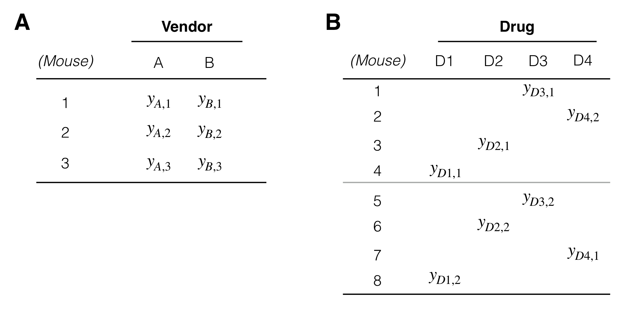
Figure 4.3: Examples of data layouts. A: Factors Vendor and Mouse are crossed. B: Factor Mouse is nested in factor Drug.

When designing an experiment, the treatment structure is determined by the purpose of the experiment: what experimental factors to consider and how to combine factor levels to treatments. The unit structure is then used to accommodate the treatment structure and to maximize precision and power for the intended comparisons. In other words:

The treatment structure is the driver in planning experiments, the design structure is the vehicle. (van Belle 2008, p180)

Finally, the experiment structure combines the treatment and unit structures and is constructed by making the randomization of each treatment on its experimental unit explicit. It provides the logical arrangement of units and treatments.

Constructing the Hasse Diagrams

To emphasize the two components of each experimental design, we draw separate Hasse diagrams for the treatment and unit structures, which we then combine into the experiment structure diagram by considering the randomization. The Hasse diagram visualizes the nesting/crossing relations between the factors. Each factor is represented by a node, shown as the factor name. If factor $B$ is nested in factor $A$, we write $B$ below $A$ and connect the two nodes with an edge. The diagram is thus ‘read’ from top to bottom. If $A$ and $B$ are crossed, we write them next to each other and connect each to the next factor that it is nested in. We then create a new factor denoted $A\!:\!B$, whose levels are the combinations of levels of $A$ with levels of $B$, and draw one edge from $A$ and one edge from $B$ to this factor. Each diagram has a top node called M or M, which represents the grand mean, and all other factors are nested in this top node.

The Hasse diagrams for our drug example are shown in Figure 4.4. The treatment structure contains the single treatment factor Drug, nested in the obligatory top node M (Fig. 4.4A). Similarly, the unit structure contains only the factor (Mouse) nested in the obligatory top node M (Fig. 4.4B).

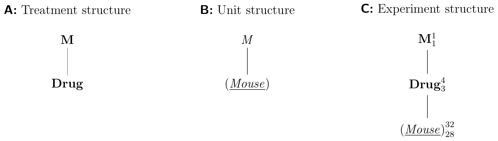
Hasse diagrams for a completely randomized design for determining effect of four different drugs using 8 mice per drug and a single response measurement per mouse.

Figure 4.4: Hasse diagrams for a completely randomized design for determining effect of four different drugs using 8 mice per drug and a single response measurement per mouse.

We construct the experiment structure diagram as follows: first, we merge the two top nodes M and M of the treatment and unit structure diagram, respectively, into a single node M. We then draw an edge from each treatment factor to its experimental unit factor. If necessary, we clean up the resulting diagram by removing unnecessary ‘shortcut’ edges: whenever there is a path $A$–$B$–$C$, we remove the edge $A$–$C$ if it exists since its nesting relation is already implied by the path.

In our example, we merge the two nodes M and M into a single node M. Both Drug and (Mouse) are now nested under the same top node. Since Drug is randomized on (Mouse), we write (Mouse) below Drug and connect the two nodes with an edge. This makes the edge from M to (Mouse) redundant and we remove it from the diagram (Fig. 4.4C).

We complete the diagram by adding the number of levels for each factor as a superscript to its node, and by adding the degrees of freedom for this factor as a subscript. The degrees of freedom for a factor $A$ are calculated as the number of levels minus the degrees of freedom of each factor that $A$ is nested in. The number of levels and the degrees of freedom of the top node M are both one.

The superscripts are the number of factor levels: 1 for M, 4 for Drug, and 32 for (Mouse). The degrees of freedom for Drug are therefore $3=4-1$, the number of levels minus the degrees of freedom of M. The degrees of freedom for (Mouse) are 28, which we calculate by subtracting from its number of levels (32) the three degrees of freedom of Drug and the single degree of freedom for M.

Hasse Diagrams and $F$-tests

We can derive the omnibus $F$-test directly from the experiment diagram in Figure 4.4C: the omnibus null hypothesis claims equality of the group means for the treatment factor Drug. This factor has four such means (given by the superscript), and the $F$-statistic has three numerator degrees of freedom (given by the subscript). For any experimental design, we find the corresponding experimental unit factor that provides the within-group variance $\sigma_e^2$ in the diagram by starting from the factor tested and moving downwards along edges until we find the first random factor. In our example, this trivially leads to identifying (Mouse) as the relevant factor, providing $N-k=28$ degrees of freedom (the subscript) for the $F$-denominator. The test thus compares $\text{MS}_\text{drug}$ to $\text{MS}_\text{mouse}$.

An Example with Subsampling

In biological experimentation, experimental units are frequently sub-sampled, and the data contain several response values for each experimental unit. In our example, we might still randomize the drug treatments on the mice, but take four blood samples instead of one from each mouse and measure them independently. Then, the mice are still the experimental units for the treatment, but the blood samples now provide the response units. The Hasse diagrams in Figure 4.5 illustrate this design.

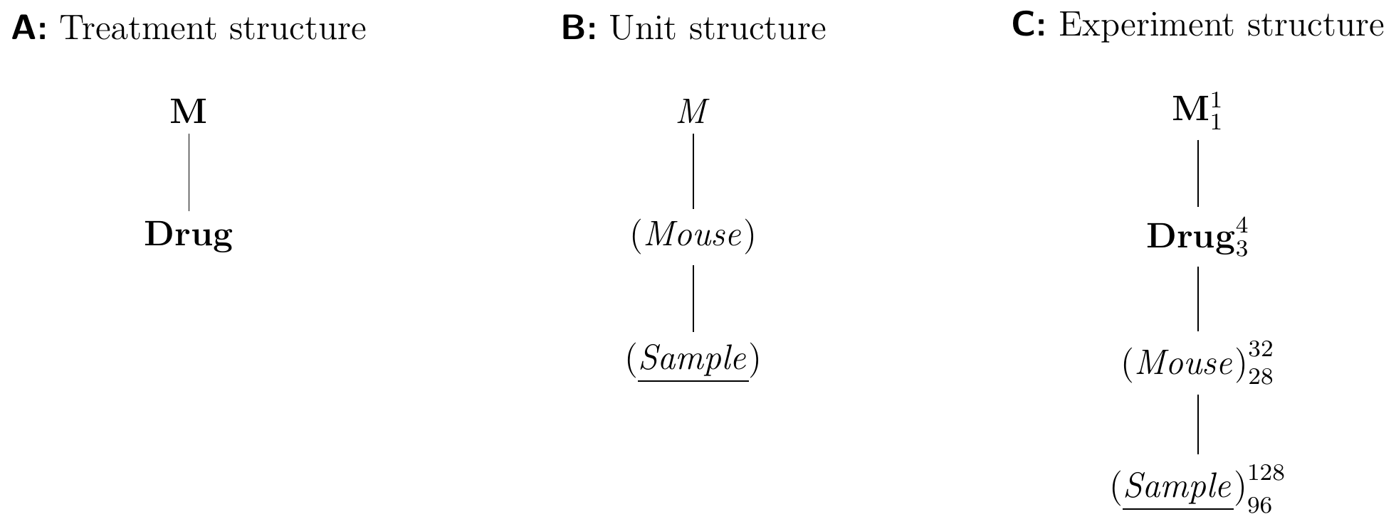
Completely randomized design for determining effect of four different drugs using 8 mice per drug and four samples measured per mouse.

Figure 4.5: Completely randomized design for determining effect of four different drugs using 8 mice per drug and four samples measured per mouse.

The treatment structure is identical to our previous example, and contains Drug as its only relevant factor. The unit structure now contains a new factor (Sample) with 128 levels, one for each measured enzyme level. It is the response factor that provides the observations. Since each sample belongs to one mouse, and each mouse has several samples, the factor (Sample) is nested in (Mouse). The observations are then partitioned first into 32 groups—one per mouse—and further into 128—one per sample per mouse. For the experiment structure, we randomize Drug on (Mouse), and arrive at the diagram in Figure 4.5C.

The $F$-test for the drug effect again uses the mean squares for Drug on 3 degrees of freedom. Using our rule, we find that (Mouse)—and not (Sample)—is the experimental unit factor that provides the estimate of the variance for the $F$-denominator on 28 degrees of freedom. As far as this test is concerned, the 128 samples are technical replicates or pseudo-replicates. They do not reflect the biological variation against which we need to test the differences in enzyme levels for the four drugs, since drugs are randomized on mice and not on samples.

4.5.2 The Linear Model

For a completely randomized design with $k$ treatment groups, we can write each datum $y_{ij}$ explicitly as the corresponding treatment group mean and a random deviation from this mean: \[\begin{equation} y_{ij} = \mu_i + e_{ij} = \mu + \alpha_i + e_{ij}\;. \tag{4.2} \end{equation}\] The first model is called a cell means model, while the second, equivalent, model is a parametric model. If the treatments had no effect, then all $\alpha_i=\mu_i-\mu$ are zero and the data are fully described by the grand mean $\mu$ and the residuals $e_{ij}$. Thus, the parameters $\alpha_i$ measure the systematic difference of each treatment from the grand mean and are independent from the experimental units.

It is crucial for an analysis that the linear model fully reflects the structure of the experiment. The Hasse diagrams allow us to derive an appropriate model for any experimental design with comparative ease. For our example, the diagram in Figure 4.4C has three factors: M, Drug, and (Mouse), and these are reflected in the three sets of parameters $\mu$, $\alpha_i$, and $e_{ij}$. Note that there are four parameters $\alpha_i$ to produce the four group means, but given three and the grand mean $\mu$, the fourth parameter can be calculated; thus, there are four parameters $\alpha_i$, but only three can be independently estimated given $\mu$, as reflected by the three degrees of freedom for Drug. Further, the $e_{ij}$ are 32 random variables, and this is reflected in the fact that (Mouse) is a random factor. Given estimates for $\mu$ and $\alpha_i$, the $e_{ij}$ in each of the four groups must sum to zero and only 28 values are independent.

For the subsampling example in Figure 4.5, the linear model is \[ y_{ijk} = \mu + \alpha_i + m_{ij} + e_{ijk}\;, \] where $m_{ij}$ is the average deviation of measurements of mouse $j$ in treatment group $i$ from the treatment group mean, and $e_{ijk}$ are the deviations of individual measurements of a mouse to its average. These terms correspond exactly to M, Drug, (Mouse), and (Sample).

4.5.3 Analysis of Variance in `R`

The aov() function provides all the necessary functionality for calculating complex ANOVAs and for estimating the model parameters of the corresponding linear models. It requires two arguments: data= indicates a data-frame with one column for each variable in the model, and aov() uses the values in these columns as the input data. The model itself is specified using a formula in the formula= argument. This formula describes the factors in the model and their crossing and nesting relationships, and can be derived directly from the experiment diagram.

For our first example, the data is stored in a data-frame called drugs which consists of 32 rows and three columns: y contains the observed enzyme level, drug the drug ($D1$ to $D4$), and mouse the number of the corresponding mouse ($1\dots 32$). Our data are then analyzed using the command aov(formula=y~1+drug+Error(mouse), data=drugs).

The corresponding formula has three parts: on the left hand side, the name of the column containing the observed response values (y), followed by a tilde. Then, a part describing the fixed factors, which we can usually derive from the treatment structure diagram: here, it contains the special symbol 1 for the grand mean $\mu$ and the term drug encoding the four parameters $\alpha_i$. Finally, the Error() part describes the random factors and is usually equivalent to the unit structure of the experiment. Here, it contains only mouse. An R formula can often be further simplified; in particular, aov() will always assume a grand mean 1, unless it is explicitly removed from the model, and will always assume that each row is one observation relating to the lowest random factor in the diagram. Both parts can be skipped from the formula and are implicitly added; our formula is thus equivalent to y~drug. We can read a formula as an instruction: explain the observations $y_{ij}$ in column y by the factors on the right: a grand mean 1 / $\mu$, the refinements drug / $\alpha_i$ that give the group means when added to the grand mean, and the residuals mouse / $e_{ij}$ that cover each difference between group mean and actual observation.

The function aov() returns a complex data structure containing the fitted model. Using summary(), we produce a human-readable ANOVA table:

m = aov(y~drug, data=drugs)
summary(m)

	Df	Sum Sq	Mean Sq	F value	Pr(>F)
drug	3	155.89	51.96	35.17	1.24e-09
Residuals	28	41.37	1.48

It corresponds to our manually computed Table 4.2. Each factor in the diagram produces one row in the ANOVA table, with the exception of the trivial factor M. Moreover, the degrees of freedom correspond between diagram factor and table row. This provides a quick and easy check if the model formula correctly describes the experiment structure. While not strictly necessary here, this is an important and useful feature of Hasse diagrams for more complex experimental designs.

From Hasse Diagram to Model Specification in `R`

From the Hasse diagrams, we construct the formula for the ANOVA as follows:

There is one variable for each factor in the diagram;
terms are added using +;
R adds the factor M implicitly; we can make it explicit by adding 1;
if factors A and B are crossed, we write A*B or equivalently A + B + A:B;
if factor B is nested in A, we write A/B or equivalently A + A:B;
the formula has two parts: one for the random factors inside the Error() term, and one for the fixed factors outside the Error() term;
in most cases, the unit structure describes the random factors and we can use its diagram to derive the Error() formula;
likewise, the treatment structure usually describes the fixed factors, and we can use its diagram to derive the remaining formula.

In our sub-sampling example (Fig. 4.5), the unit structure contains (Sample) nested in (Mouse) and we describe this nesting by the formula mouse/sample. The formula for the model is thus y~1+drug+Error(mouse/sample), respectively y~drug+Error(mouse).

The aov() function does not directly provide estimates of the group means, and an elegant way of estimating them in R is the emmeans() function from the emmeans package.¹ It calculates the expected marginal means (sometimes confusingly called least-squares means) as defined in (Searle, Speed, and Milliken 1980) for any combination of experiment factors using the model found by aov(). In our case, we can request the estimated group averages $\hat{\mu}_i$ for each level of drug, which emmeans() calculates from the model as $\hat{\mu}_i = \hat{\mu} + \hat{\alpha}_i$:

em = emmeans(m, ~drug)

This yields the estimates, their standard errors, degrees of freedom, and 95%-confidence intervals in Table 4.3.

Table 4.3: Estimated cell means, standard errors and 95%-confidence intervals.
	Mean	se	df	LCL	UCL
D1	14.33	0.43	28	13.45	15.21
D2	12.81	0.43	28	11.93	13.69
D3	9.24	0.43	28	8.36	10.12
D4	9.34	0.43	28	8.46	10.22

4.6 Unbalanced Data

When designing an experiment with a single treatment factor, it is rather natural to consider using the same number of experimental units for each treatment group. We saw in Section 3.2 that this also leads to the lowest possible standard error when estimating the difference between any two treatment means, provided that the ANOVA assumption of equal variance in each treatment group holds.

Sometimes, such a fully balanced design is not achieved, because the number of available experimental units is not a multiple of the number of treatment groups. For example, we might consider studying the four drugs again, but with only 30 mice at our disposal rather than 32. Then, we either need to reduce each treatment group to seven mice, leaving two mice, or use eight mice in two treatment groups, and seven in the other two (alternatively eight mice in three groups and six in the remaining).

Another cause for missing full balance is that some experimental units fail to give usable response values during the experiment or their recordings go missing. This might happen because some mice die (or escape) during the experiment, a sample gets destroyed or goes missing, or some faulty readings are discovered after the experiment is finished.

In either case, the number of responses per treatment group is no longer the same number $n$, but each treatment group has its own number of experimental units $n_i$, with total experiment size $N=n_1+\cdots+n_k$ for $k$ treatment groups.

4.6.1 Analysis of Variance

The one-way analysis of variance is little influenced by unbalanced data, provided each treatment group has at least one observation. The total sum of squares again decomposes into a treatment and a residual term, both of which now depend on the $n_i$ in the obvious way: \[ \text{SS}_\text{tot} = \sum_{i=1}^k\sum_{j=1}^{n_i}(y_{ij}-\bar{y}_i+\bar{y}_i-\bar{y})^2 = \underbrace{\sum_{i=1}^k n_i\cdot (\bar{y}_i-\bar{y})^2}_{\text{SS}_\text{trt}} + \underbrace{\sum_{i=1}^k\sum_{j=1}^{n_i} (y_{ij}-\bar{y}_i)^2}_{\text{SS}_\text{res}} \;. \] Clearly, if no responses are observed for a treatment group, its average response cannot be estimated, and no inference is possible about this group or its relation to other groups.

The ratio of treatment to residual mean squares then again forms the $F$-statistic \[ F = \frac{\text{SS}_{\text{trt}}/(k-1)}{\text{SS}_{\text{res}}/(N-k)} \] which has an $F$-distribution with $k-1$ and $N-k$ degrees of freedom under the null hypothesis $H_0: \mu_1=\cdots =\mu_k$ that all treatment group means are equal.

4.6.2 Estimating the Grand Mean

With unequal numbers $n_i$ of observations per cell, we now have two reasonable estimators for the grand mean $\mu$: one estimator is the weighted mean $\bar{y}_{\bigcdot\bigcdot}$, which is the direct equivalent to our previous estimator: \[ \bar{y}_{\bigcdot\bigcdot} =\frac{y_{\bigcdot\bigcdot}}{N} = \frac{1}{N}\sum_{i=1}^k\sum_{j=1}^{n_i}y_{ij} = \frac{n_1\cdot \bar{y}_{1\bigcdot}+\cdots n_a\cdot \bar{y}_{k\bigcdot}}{n_1+\cdots +n_k} = \frac{n_1}{N} \cdot \bar{y}_{1\bigcdot}+ \cdots +\frac{n_k}{N}\cdot \bar{y}_{k\bigcdot}\;. \] This estimator weighs each estimated treatment group mean by the number of available response values and hence its value depends on the number of observations per group via the weights $n_i/N$. Its variance is \[ \text{Var}(\bar{y})=\frac{\sigma^2}{N}\;. \]

The weighted mean is often an undesirable estimator, because larger groups then contribute more to the estimation of the grand mean. In contrast, the unweighted mean \[ \tilde{y}_{\bigcdot\bigcdot} = \frac{1}{k}\sum_{i=1}^k \left(\frac{1}{n_i}\sum_{j=1}^{n_i}y_{ij}\right) = \frac{\bar{y}_{1\bigcdot}+\cdots+ \bar{y}_{k\bigcdot}}{k} \] first calculates the average of each treatment group based on the available observations, and then takes the mean of these group averages as the grand mean. This is precisely the estimated marginal mean, an estimator for the population marginal mean $\mu=(\mu_1+\cdots +\mu_k)/k$.

In direct extension to our discussion in Section 3.2, its variance is \[ \text{Var}(\tilde{y}_{\bigcdot\bigcdot})=\frac{\sigma^2}{k^2}\cdot\left(\frac{1}{n_1}+\cdots +\frac{1}{n_k}\right)\;, \] which is minimal if $n_1=\cdots =n_k$ and then reduces to the familiar $\sigma^2/N$.

These two estimators yield the same result if the data are balanced and $n_1=\cdots =n_k$, but their estimates differ for unbalanced data. For example, taking the first 4, 2, 1, and 2 responses for $D1$, $D2$, $D3$, and $D4$ from Table 4.1 yields a fairly unbalanced design in which $D3$ (with comparatively low responses) is very underrepresented compared to $D1$ (with high value), for example. The two estimators are $\bar{y}_{\bigcdot\bigcdot}=$ 12.5 and $\tilde{y}_{\bigcdot\bigcdot}=$ 11.84. The average on the full data is 11.43.

4.6.3 Degrees of Freedom

With different numbers of observations between groups, the resulting degrees of freedom with $k$ treatment groups and a total of $N$ observations are still $k-1$ for the treatment factor, and $N-k$ for the residuals for designs without subsampling. If subsampling of experimental units is part of the design, however, the degrees of freedom in the $F$-test statistic can no longer be determined exactly. A common approximation is the conceptually simple Satterthwaite approximation based on a weighted mean (Satterthwaite 1946), while the more conservative Kenward-Roger approximation (Kenward and Roger 1997) provides degrees of freedom that agree with the Hasse diagram for more complex models that we discuss later.

4.7 Notes and Summary

Notes

Standard analysis of variance requires normally distributed, independent data in each treatment group, and homogeneous group variances. Moderate deviations from normality and moderately unequal variances have little impact on the $F$-statistics, but non-independence can have devastating effects (Cochran 1947; Lindman 1992). The method by Kruskal and Wallis provides an alternative to the one-way ANOVA based on ranks of observations rather than an assumption of normally distributed data (Kruskal and Wallis 1952).

Effect sizes for ANOVA are comparatively common in psychology and related fields (Cohen 1988; Lakens 2013), but have also been advertised for biological sciences, where they are much less used (Nakagawa and Cuthill 2007). Like any estimate, standardized effect sizes should also be reported with a confidence interval, but standard software rarely provides out-of-the-box calculations (Kelley 2007); these confidence intervals are calculated based on noncentral distributions, similar to our calculations in Section 2.5 for Cohen’s $d$ (W. Venables 1975; Cumming and Finch 2001). The use of its upper confidence limit rather than the variance’s point estimate for power analysis is evaluated in Kieser and Wassmer (1996). A pilot study can be conducted to estimate the variance and enable informed power calculations for the main experiment; a group size of $n=12$ is recommended for clinical pilot trials (Julious 2005). The use of portable power analysis makes use of $\phi^2$ for which tables were originally given in Tang (1938).

A Simple Function for Calculating Sample Size

The following code illustrates the power calculations from Section 4.4. It accepts a variety of effect size measures ($b^2$, $f^2$, $\eta^2$, or $\lambda$), either the numerator degrees of freedom df1= or the number of treatment groups k=, the denominator degrees of freedom df2= or the number of samples n=, and the significance level alpha= and calculates the power of the omnibus $F$-test. This code is meant to be more instructional than practical, but its more versatile arguments will also allow us to perform power analysis for linear contrasts, which is not possible with the built-in power.anova.test(). For a sample size calculation, we would start with a small $n$, use this function to find the power, and then increment $n$ until the desired power is exceeded.

# Provide EITHER b2 (with s) OR f2 OR lambda OR eta2
# Provide EITHER k OR df1,df2
getPowerF = function(n, k=NULL, df1=NULL, df2=NULL, 
                     b2=NULL, s=NULL, 
                     f2=NULL, lambda=NULL, eta2=NULL, 
                     alpha) {
  # If necessary, calculate degrees of freedom
  if(is.null(df1)) df1 = k - 1
  if(is.null(df2)) df2 = n*k - k
  # Map effect size to ncp lambda=f2*n*k if necessary
  if(!is.null(b2)) lambda = b2 * n * (df1+1) / s
  if(!is.null(f2)) lambda = f2 * n * (df1+1)
  if(!is.null(eta2)) lambda = (eta2 / (1-eta2)) * n * (df1+1)
  # Critical quantile for rejection under H0
  q = qf(p=1-alpha, df1=df1, df2=df2)
  # Power
  pwr = 1 - pf(q=q, ncp=lambda, df1=df1, df2=df2)
  return(pwr)
}

ANOVA and Linear Regression

The one-way ANOVA is formally equivalent to a linear regression model with regressors $x_{1j},\dots,x_{kj}$ to encode the $k$ group memberships: \[ y_{ij} = \mu + \alpha_i + e_{ij} = \mu + \alpha_1\cdot x_{1j} + \cdots + \alpha_k\cdot x_{kj} + e_{ij}\;, \] and this model is used internally by R. Since it describes $k$ group means $\mu_1,\dots,\mu_k$ by $k+1$ parameters $\mu,\alpha_1,\dots,\alpha_k$, it is overparameterized and an additional constraint is required for finding suitable estimates (Nelder 1994, 1998). Two common constraints are the treatment coding and the sum coding which both yield (dependent) parameter estimates, but these estimates will differ in value and in interpretation. For this reason, we only use the linear model fit to calculate the estimated marginal means, such as group averages, which are independent of the coding for the parameters used in the model estimation procedure.

The treatment coding uses $\hat{\alpha}_r=0$ for a specific reference group $r$; $\hat{\mu}$ then estimates the group mean of the reference group $r$ and $\hat{\alpha}_i$ estimates the difference between group $i$ and the reference group $r$. The vector of regressors for the response $y_{ij}$ is \[\begin{align*} (x_{1j},\dots,x_{kj}) &= (0,\dots,0,\underbrace{1}_i,0,\dots,0) \text{ for } i\not= r \\ (x_{1j},\dots,x_{kj}) &= (0,\dots,0,\underbrace{0}_i,0,\dots,0) \text{ for } i= r\;. \end{align*}\] In R, the treatment groups are usually encoded as a factor variable, and aov() will use its alphabetically first level as the reference group by default. We can set the reference level manually using relevel() in base-R or the more convenient fct_relevel() from the forcats package. We can use the dummy.coef() function to extract all parameter estimates from the fitted model, and summary.lm() to see the estimated parameters together with their standard errors and $t$-tests. The treatment coding can also be set manually using the contrasts= argument of aov() together with contr.treatment(k), where k is the number of treatment levels.

For our example, aov() uses the treatment level $D1$ as the reference level. This gives the estimates (Intercept) $=\hat{\mu}=$ 14.33 for the average enzyme level in the reference group, which serves as the grand mean, $D1=\hat{\alpha}_1=$ 0 as expected, and the three differences from $D2$, $D3$, and $D4$ to $D1$ as $D2=\hat{\alpha}_2=$ $-1.51$, $D3=\hat{\alpha}_3=$ $-5.09$, and $D4=\hat{\alpha}_4=$ $-4.99$, respectively. We find the group mean for $D3$, for example, as $\hat{\mu}_3=\hat{\mu}+\hat{\alpha}_3=$ 14.33 + $(-5.09)$ = 9.24.

The sum coding uses the constraint $\sum_{i=1}^k \hat{\alpha}_i = 0$. Then, $\hat{\mu}$ is the estimated grand mean, and $\hat{\alpha}_i$ is the estimated deviation of the $i$th group mean from this grand mean. The vector of regressors for the response $y_{ij}$ is \[\begin{align*} (x_{1j},\dots,x_{kj}) &= (0,\dots,0,\underbrace{1}_i,0,\dots,0) \text{ for } i=1,\dots,k-1 \\ (x_{1j},\dots,x_{kj}) &= (-1,\cdots,-1, 0) \text{ for } i=k\;. \\ \end{align*}\] The aov() function uses the argument contrasts= to specify the desired coding for each factor, and contrasts=list(drug=contr.sum(4)) provides the sum encoding for our example. The resulting parameter estimates are (Intercept) $=\hat{\mu}=$ 11.43 for the average enzyme level over all groups, and $D1=\hat{\alpha}_1=$ 2.9, $D2=\hat{\alpha}_2=$ 1.38, $D3=\hat{\alpha}_3=$ $-2.19$, and $D4=\hat{\alpha}_4=$ $-2.09$, respectively, as the specific differences from each estimated group mean to the estimated general mean. As required, the estimated differences add to zero and we find the group mean for $D3$ as $\hat{\mu}_3=\hat{\mu}+\hat{\alpha}_3=$ 11.43 + $(-2.19)$ = 9.24.

Using `R`

Base-R provides the aov() function for calculating an analysis of variance. The model is specified using R’s formula framework, which implements a previously proposed symbolic description of models (Wilkinson and Rogers 1973). The summary() function prints the ANOVA table of a fitted model. Alternatively, the same model specification (but without Error()) can be used with the linear regression function lm() in which case summary() provides the (independent) regression parameter estimates and dummy.coef() gives a list of all parameters. The functions summary.lm() and summary.aov() provide the respective other view for these two equivalent models. Further details are provided in Section 4.5.3.

ANOVA tables can also be calculated from other types of regression models (we look at linear mixed models in subsequent chapters) using the function anova() with the fitted model. This function also allows specifying the approximation method for calculating degrees of freedom using its ddf= option. Power analysis for a one-way ANOVA is provided by power.anova.test(). Completely randomized experiments can be designed using design.crd() from package agricolae, which also provides randomization.

Exact confidence limits for $f^2$ and $\eta^2$ are translated from those calculated for the noncentrality parameter $\lambda$ of the $F$-distribution. The effectsize package provides functions cohens_f() and eta_squared() for calculating these effect sizes and their confidence intervals.

Summary

The analysis of variance decomposes the overall variation in the data into parts attributable to different sources, such as treatment factors and residuals. The decomposition relies on a partition of the sum of squares, measuring the variation, and the degrees of freedom, measuring the amount of data expended on each source. The ANOVA table provides a summary of this decomposition: sums of squares and degrees of freedom for each source, and the resulting mean squares. The $F$-test compares two variance estimates, provided by mean squares terms, and comparing the mean squares of a treatment to the residual mean squares tests the hypothesis that all group means are equal. For two groups, this is equivalent to a $t$-test with equal group variances.

Hasse diagrams visualize the logical structure of an experiment: we distinguish the unit structure with the unit factors and their relations from the treatment structure with the treatment factors and their relations. We combine both into the experiment structure by linking each treatment factor to the unit factor on which it is randomized; this is the experimental unit for that treatment factor and provides the residual mean squares of the $F$-test. We derive the model specification directly from the Hasse diagram and can verify correct specification by comparing the degrees of freedom from the diagram with those in the resulting ANOVA table.

This package was previously called lsmeans (Lenth 2016).↩︎