Chapter 3 Planning for Precision and Power

3.1 Introduction

In our original two-vendor example, we found that twenty mice were insufficient to conclude if the two kits provide comparable measurements on average or not. We now discuss several methods for increasing precision and power by reducing the standard error: (i) balancing allocation of a fixed number of samples to the treatment groups; (ii) reducing the standard deviation of the responses; and (iii) increasing the sample size. The sample size required for desired precision and power is determined by power analysis.

3.2 Balancing Allocation

Without comment, we always used a balanced allocation, where the same number of experimental units is allocated to each treatment group. This choice seems intuitively sensible, and we quickly confirm that it indeed yields the highest precision and power in our example. We will later see that unbalanced allocation not only decreases precision, but might prevent estimation of relevant treatment effects altogether in more complex designs.

We denote by \(n_A\) and \(n_B\) the number of mice allocated to kit A and B, respectively. The standard error of our estimate is then \[ \text{se}(\hat{\mu}_A-\hat{\mu}_B) = \sqrt{\frac{1}{n_A}+\frac{1}{n_B}}\cdot\sigma\;, \] where we estimate the two expectations by \(\hat{\mu}_A=\sum_{i=1}^{n_A}y_{i,A}/n_A\) and correspondingly for \(\hat{\mu}_B\).

For fixed total sample size \(n_A+n_B\), this standard error is minimal for a balanced allocation with treatment groups of equal size \(n_A=n_B\), provided the variance \(\sigma^2\) is identical in both treatment groups. The more unbalanced the allocation is, the larger the standard error will become.

To illustrate, we consider two experimental designs with a total sample size of \(n_A+n_B=20\): first, we assign a single mouse to vendor B (\(n_B=1\)), and the remaining mice to vendor A (\(n_A=19\)). Then, \[ \text{se}_{19,1} = \sqrt{\frac{1}{19}+\frac{1}{1}}\cdot\sigma = 1.026\,\sigma \] and the standard error is even higher than the dispersion in the population! However, if we assign the mice equally (\(n_A=n_B=10\)), we get a substantially lower standard error of \[ \text{se}_{10,10} = \sqrt{\frac{1}{10}+\frac{1}{10}}\cdot\sigma = 0.45\,\sigma\;. \]

The relative efficiency of the two designs \[ \text{RE} = \frac{\text{se}_{19,1}^2}{\text{se}_{10,10}^2} = \left(\frac{1.026\,\sigma}{0.45\,\sigma}\right)^2 \approx 5.2 \] allows us to directly compare the precision of the two allocation strategies. It is the increase in sample size needed for the first experiment to match the precision of the second. Here, the same unbalanced allocation would require about five times more mice to match the precision of the balanced design. This would mean using at least 5 mice for vendor B and 95 mice for vendor A (100 mice in total). Dividing the experimental material inaptly results in substantial loss of precision, which is very costly to make up for.

If the two treatment groups have very different standard deviations \(\sigma_A\) and \(\sigma_B\), then the standard error is \[ \text{se}(\hat{\mu}_A-\hat{\mu}_B) = \sqrt{\frac{\sigma_A^2}{n_A}+\frac{\sigma_B^2}{n_B}}\;. \]

The standard error is minimal if \(\sigma_A/n_A\approx \sigma_B/n_B\) and we should allocate the samples proportionally to the standard deviation in each group. For \(n_A+n_B=20\) mice and \(\sigma_A=2.8\) twice as large as \(\sigma_B=1.4\), we then allocate \(n_A=\) 13 and \(n_B=\) 7 mice, respectively, and use \(n_A=\) 16 and \(n_B=\) 4 mice if the standard deviation in group A is \(\sigma_A=5.6\). Very disparate standard errors in the different treatment groups are often a sign that the treatment groups are different in ways other than the assigned treatment alone; such a situation will require more care in the statistical analysis.

3.3 Reducing the Standard Error

We can increase precision and power by reducing the standard deviation \(\sigma\) of our response values. This option is very attractive, since reducing \(\sigma\) to one-half will also cut the standard error to one-half and increase the value of the \(t\)-statistic by two, without altering the necessary sample size.

Recall that the standard deviation describes how dispersed the measured enzyme levels of individual mice are around the population mean in each treatment group. This dispersion contains the biological variation \(\sigma_m\) from mouse to mouse, and the variation \(\sigma_e\) due to within-mouse variability and measurement error, such that \[ \sigma^2=\sigma_m^2+\sigma_e^2 \quad\text{and}\quad \text{se}(\hat{\Delta}) = \sqrt{2\cdot\left( \frac{\sigma_m^2+\sigma_e^2}{n}\right)} \;. \]

3.3.1 Sub-sampling

If the variance \(\sigma^2\) is dominated by variation between samples of the same mouse, we can reduce the standard error by taking multiple samples from each mouse. Averaging their measured enzyme levels estimates each mouse’s response more precisely. Since the number of experimental units does not change, the measurements from the samples are sometimes called technical replicates as opposed to biological replicates. If we take \(m\) samples per mouse, this reduces the variance of these new responses to \(\sigma_m^2+\sigma_e^2/m\), and the standard error to \[ \text{se}(\hat{\Delta}) = \sqrt{ 2\cdot \left(\frac{\sigma_m^2}{n}+\frac{\sigma_e^2}{m\cdot n}\right)}\;. \] We can employ the same strategy if the measurement error is large, and we decrease its influence on the standard error by taking \(r\) measurements of each of \(m\) samples.

This strategy is called sub-sampling and is only successful in increasing precision and power substantially if \(\sigma_e\) is not small compared to the between-mouse variation \(\sigma_m\), since the contribution of \(\sigma_m\) on the standard error only depends on the number \(n\) of mice, and not on the number \(m\) of samples per mouse. In biological experiments, the biological (mouse-to-mouse) variation is typically much larger than the technical (sample-to-sample) variation and sub-sampling is of very limited use. Indeed, a very common mistake is to ignore the difference between technical and biological replicates and treat all measurements as biological replicates. This flaw is known as pseudo-replication and leads to overestimating the precision of an estimate and thus to much shorter, incorrect, confidence intervals, and to overestimating the power of a test, with too low \(p\)-values and high probability of false positives (Hurlbert 1984, 2009).

For our examples, the between-mouse variance is \(\sigma_m^2=\) 1.9 and much larger than the within-mouse variance \(\sigma_e^2=\) 0.1. For \(n=10\) mice per treatment group and \(m=1\) samples per mouse, the standard error is 0.89. Increasing the number of samples to \(m=2\) reduces this error to 0.88 and further increasing to an unrealistic \(m=100\) only reduces the error down to 0.87. In contrast, using 11 instead of 10 mice per treatment reduces the standard error already to 0.85.

3.3.2 Narrowing the Experimental Conditions

We can reduce the standard deviation \(\sigma\) of the observations by tightly controlling experimental conditions, for example by keeping temperatures and other environmental factors at a specific level, reducing the diversity of the experimental material, and similar measures.

For our examples, we can reduce the between-mouse variation \(\sigma_m\) by restricting attention to a narrower population of mice. If we sample only female mice within a narrow age span from a particular laboratory strand, the variation might be substantially lower than for a broader selection of mice.

However, by ever more tightly controlling the experimental conditions, we simultaneously restrict the generalizability of the findings to the narrower conditions of the experiment. Claiming that the results should also hold for a wider population (i.e., other age cohorts, male mice, more than one laboratory strand) requires external arguments and cannot be supported by the data from our experiment.

3.3.3 Blocking

Looking at our experimental question more carefully, we discovered a simple yet highly efficient technique to completely remove the largest contributor \(\sigma_m\) from the standard error. The key observation is that we apply each kit to a sample from a mouse and not to the mouse directly. Rather than taking one sample per mouse and randomly allocating it to either kit, we can also take two samples from each mouse, and randomly assign kit A to one sample, and kit B to the other sample (Figure 1.1C). For each mouse, we estimate the difference between vendors by subtracting the two measurements, and average these differences over the mice. Each individual difference is measured under very tight experimental conditions (within a single mouse); provided the differences vary randomly and independently of the mouse (note that the measurements themselves of course depend on the mouse!), their average yields a within-mouse estimate for \(\hat{\Delta}\).

Such an experimental design is called a blocked design, where the mice are blocks for the samples: they group the samples into pairs belonging to the same mouse, and treatments are independently randomized to the experimental units within each group. This effectively removes the variation between blocks from the treatment comparison, as we saw in Section 2.3.5.3.

If we consider our paired-vendor example again, each observation has variance \(\sigma_m^2+\sigma_e^2\), and the two treatment group mean estimates \(\hat{\mu}_A\) and \(\hat{\mu}_B\) both have variance \((\sigma_m^2+\sigma_e^2)/n\). However, the estimate \(\hat{\Delta}=\hat{\mu}_A-\hat{\mu}_B\) of their difference only has variance \(2\cdot\sigma_e^2/n\), and the between-mouse variance \(\sigma_m^2\) is completely eliminated from this estimate. This is because each observation from the same mouse is equally affected by any systematic deviation that exist between the specific mouse and the overall average, and this deviation therefore cancels if we look at differences between observations from the same mouse.

For \(\sigma_m^2=\) 1.9 and \(\sigma_e^2=\) 0.1, for example, blocking by mouse reduces the expected standard error from 0.89 in the original two-vendor experiment to 0.2 in the paired-vendor experiment. Simultaneously, the experiment size is reduced from 20 to 10 mice, while the number of observations remains the same. Importantly, the samples—and not the mice—are the experimental units in this experiment, since we randomly assign kits to samples and not to mice. In other words, we still have 20 experimental units, the same as in the original experiment.

The relative efficiency between unblocked experiment and blocked experiment is \(\text{RE}=\) 20, indicating that blocking allows a massive reduction in sample size while keeping the same precision and power.

As expected, the \(t\)-test equally profits from the reduced standard error. The \(t\)-statistic is now \(t=-2.9\) leading to a \(p\)-value of \(p=\) 0.018 and thus a significant result at the 5%-significance level. This compares to the previous \(t\)-value of \(t=-0.46\) for the unblocked design with a \(p\)-value of 0.65.

3.4 Sample Size and Precision

“How many samples do I need?” is arguably among the first questions a researcher asks when thinking about an experimental design. Sample size determination is a crucial component of experimental design in order to ensure that estimates are sufficiently precise to be of practical value and that hypothesis tests are adequately powered to be able to detect a relevant effect size. Sample size determination crucially depends on deciding on a minimal effect size. While precision and power can always be increased indefinitely by increasing the sample size, limits on resources—time, money, available experimental material—pose practical limits. There is also a diminishing return, as doubling precision requires quadrupling the sample size.

3.4.1 Sample Size for Desired Precision

To provide a concrete example, let us consider our comparison of the two preparation kits again and assume that the volume of blood required is prohibitive for more than one sample per mouse. In the two-vendor experiment based on 20 mice, we found that our estimate \(\hat{\Delta}\) was too imprecise to determine with any confidence which—if any—of the two kits yields lower responses than the other.

To determine a sufficient sample size, we need to decide which minimal effect size is relevant for us, a question answerable only with experience and subject-matter knowledge. For the sake of the example, let us say that a difference of \(\delta_0=\pm 0.5\) or larger would mean that we stick with one vendor, but a smaller difference is not of practical relevance for us. The task is therefore to determine the number \(n\) of mice per treatment group, such that the confidence interval of \(\Delta\) has width no more than one, i.e., that \[\begin{align*} \text{UCL}-\text{LCL} &= (\hat{\Delta}+t_{1-\alpha/2,2n-2}\cdot\text{se}(\hat{\Delta}))-(\hat{\Delta}+t_{\alpha/2,2n-2}\cdot\text{se}(\hat{\Delta})) \\ & = (t_{1-\alpha/2,2n-2}-t_{\alpha/2,2n-2})\cdot\sqrt{2}\sigma/\sqrt{n} \\ & \leq 2|\delta_0| \;. \end{align*}\] We note that the \(t\)-quantiles and the standard error both depend on \(n\), which prevents us from solving this inequality directly. For a precise calculation, we can start at some not too large \(n\), calculate the width of the confidence interval, increase \(n\) if the width is too large, and repeat until the desired precision is achieved.

If we have reason to believe that \(n\) will not be very small, then we can reduce the problem to \[ \text{UCL}-\text{LCL} = (z_{1-\alpha/2}-z_{\alpha/2})\sqrt{2}\sigma/\sqrt{n} \leq 2|\delta_0| \implies n\geq 2\cdot z_{1-\alpha/2}^2\sigma^2/\delta_0^2\;, \] if we exploit the fact that the \(t\)-quantile \(t_{\alpha,n}\) is approximately equal to the standard normal quantile \(z_\alpha\), which does not depend on the sample size.

For a 95%-confidence interval we have \(z_{0.975}=+1.96\), which we can approximate as \(z_{0.975}\approx 2\) without introducing any meaningful error. This leads to the simple formula \[ n \geq 8\sigma^2/\delta_0^2\;. \]

In order to actually calculate the sample size with this formula, we need to know the standard deviation of the enzyme levels or an estimate \(\hat{\sigma}\). Such an estimate might be available from previous experiments on the same problem. If not, we have to conduct a separate (usually small) experiment using a single treatment group for getting such an estimate. In our case, we already have an estimate \(\hat{\sigma}=\) 1.65 from our previous experiment, from which we find that a sample size of \(n=\) 84 mice per kit is required to reach our desired precision (the approximation \(z_{0.975}=2\) yields \(n=\) 87). This is a substantial increase in experimental material needed. We will have to decide if an experiment of this size is feasible for us, but a smaller experiment will likely waste time and resources without providing a practically relevant answer.

3.4.2 Precision for Given Sample Size

It is often useful to turn the question around: given we can afford a certain maximal number of mice for our experiment, what precision can we expect? If this precision turns out to be insufficient for our needs, we might as well call the experiment off or start considering alternatives.

For example, let us assume that we have 40 mice at our disposal for the experiment. From our previous discussion, we know that the variances of measurements using kits A and B can be assumed equal, so a balanced assignment of \(n=20\) mice per vendor is optimal. The expected width of a 95%-confidence interval is \[ \text{UCL}-\text{LCL} = (z_{0.975}-z_{0.025})\cdot\sqrt{2}\sigma/\sqrt{n} = 1.24\cdot\sigma\;. \] Using our previous estimate of \(\hat{\sigma}=\) 1.65, we find the expected width of the 95%-confidence interval of 2.05 compared to 2.9 for the previous experiment with 10 mice per vendor, a decrease in length by \(\sqrt{2}=1.41\) due to doubling the sample size. This is not even close to our desired length of one, and we should consider if this experiment is worth doing, since it uses resources without a reasonable chance of providing a precise-enough estimate.

3.5 Sample Size and Power

A more common approach for determining the required sample size is via a hypothesis testing framework and allows us to also consider acceptable false positive and false negative probabilities for our experiment. For any hypothesis test, we can calculate each of the following five parameters from the other four:

• The sample size \(n\).
• The minimal effect size \(\delta_0\) we want to reliably detect: the smaller the minimal effect size, the more samples are required to distinguish it from a zero effect. It is determined by subject-matter considerations and both raw and standardized effect sizes can be used.
• The variance \(\sigma^2\): the larger the variance of the responses, the more samples we need to average out random fluctuations and achieve the necessary precision. Reducing the variance using the measures discussed above always helps, and blocking in particular is a powerful design option if available.
• The significance level \(\alpha\): the more stringent this level, the more samples we need to reliably detect a given effect. In practice, values of 5% or 1% are common.
• The power \(1-\beta\): this probability is higher the more stringent our \(\alpha\) is set (for a fixed difference) and larger effects will lead to fewer false negatives for the same \(\alpha\) level. In practice, the desired power is often about 80–90%; higher power might require prohibitively large sample sizes.

3.5.1 Power Analysis for Known Variance

We start developing the main ideas for determining a required sample size in a simplified scenario, where we know the variance exactly. Then, the standard error of \(\hat{\Delta}\) is also known exactly, and the test statistic \(\hat{\Delta}/\text{se}(\hat{\Delta})\) has a standard normal distribution under the null hypothesis \(H_0: \Delta=0\). The same calculations can also be used with a variance estimate, provided the sample size is not too small and the \(t\)-distribution of the test statistic is well approximated by the normal distribution.

In the following, we assume that we decided on the false positive probability \(\alpha\), the power \(1-\beta\), and the minimal effect size \(\Delta=\delta_0\). If the true difference is smaller than \(\delta_0\), we might still detect it, but detection becomes less and less likely the smaller the difference gets. If the difference is greater, our chance of detection increases.

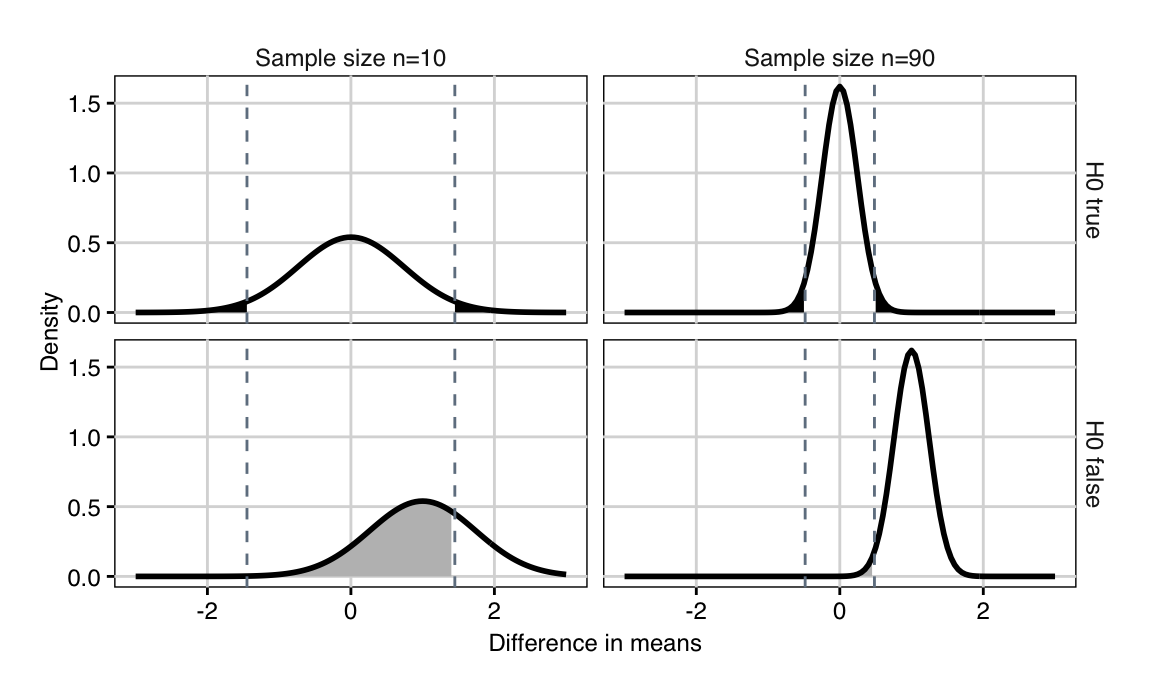
Figure 3.1: Distributions of difference in means if null hypothesis is true and difference between means is zero (top) and when alternative hypothesis is true and difference is one (bottom) for 10 (left) and 90 (right) samples. The dashed lines are the critical values for the test statistic. Shaded black region: false positives (\(\alpha\)). Shaded grey region: false negatives (\(\beta\)).

If \(H_0: \Delta=0\) is true, then \(\hat{\Delta}\sim N(0,2\sigma^2/n)\) has a normal distribution with mean zero and variance \(2\sigma^2/n\). We reject the null hypothesis if \(\hat{\Delta}\leq z_{\alpha/2}\cdot \sqrt{2}\sigma/\sqrt{n}\) or \(\hat{\Delta}\geq z_{1-\alpha/2}\cdot \sqrt{2}\sigma/\sqrt{n}\). These two critical values are shown as dashed vertical lines in Figure 3.1 (top) for sample sizes \(n=\) 10 (left) and \(n=\) 90 (right). As expected, the critical values move closer to zero with increasing sample size.

If \(H_0\) is not true and \(\Delta=\delta_0\) instead, then \(\hat{\Delta}\sim N(\delta_0,2\sigma^2/n)\) has a normal distribution with mean \(\delta_0\) and variance \(2\sigma^2/n\). This distribution is shown in the bottom row of Figure 3.1 for the two sample sizes and a true difference of \(\delta_0=\) 1; it also gets narrower with increasing sample size \(n\).

A false negative happens if \(H_0\) is not true, so \(\Delta=\delta_0\), yet the estimator \(\hat{\Delta}\) falls outside the rejection region. The probability of this event is \[ \mathbb{P}\left( |\hat{\Delta}|\leq z_{1-\alpha/2}\cdot\frac{\sqrt{2}\cdot\sigma}{\sqrt{n}}; \Delta=\delta_0 \right) = \beta\;, \] which yields the fundamental equality \[\begin{equation} z_{1-\alpha/2}\cdot \sqrt{2}\sigma / \sqrt{n} = z_{\beta}\cdot \sqrt{2}\sigma / \sqrt{n}+\delta_0\;. \tag{3.1} \end{equation}\] Our goal is to find \(n\) such that the probability of a false negative stays below a prescribed value \(\beta\).

We can see this in Figure 3.1: for a given \(\alpha=5\%\), the dashed lines denote the rejection region, and the black shaded area has probability 5%. If \(\Delta=\delta_0\), we get the distributions in the bottom row, where all values inside the dashed lines are false negatives, and the probability \(\beta\) corresponds to the grey shaded area. Increasing \(n\) from \(n=\) 10 (left) to \(n=\) 90 (right) narrows both distributions, moves the critical values towards zero, and shrinks the false negative probability.

We find a closed formula for the sample size by solving Equation (3.1) for \(n\): \[\begin{equation} n = \frac{2\cdot(z_{1-\alpha/2}+z_{1-\beta})^2}{(\delta_0/\sigma)^2} = \frac{2\cdot(z_{1-\alpha/2}+z_{1-\beta})^2}{d_0^2} \tag{3.2}\;, \end{equation}\] where we used the fact that \(z_{\beta}=-z_{1-\beta}\). The first formula uses the minimal raw effect size \(\delta_0\) and requires knowledge of the residual variance, whereas the second formula is based on the minimal standardized effect size \(d_0=\delta_0/\sigma\), which measures the difference between the means as a multiple of the standard deviation.

In our example, a hypothesis test with significance level \(\alpha=5\%\) and a variance of \(\sigma^2=\) 2 has power 11%, 35%, and 100% to detect a true difference of \(\delta_0=\) 1 based on \(n=2\), \(n=10\), and \(n=100\) mice per treatment group, respectively. We require at least 31 mice per vendor to achieve a power of \(1-\beta=80\%\).

The same ideas apply to calculating the minimal effect size that is detectable with given significance level and power for any fixed sample size. For our example, we might only have 20 mice per vendor at our disposal. For our variance of \(\sigma^2=\) 2, a significance level of \(\alpha=5\%\) and a power of \(1-\beta=80\%\), we find that for \(n=20\), the achievable minimal effect size is \(\delta_0=\) 1.25.

A small minimal standardized effect size of \(d_0=\delta_0/\sigma=0.2\) requires at least \(n=\) 392 mice per vendor for \(\alpha=5\%\) and \(1-\beta=80\%\). This number decreases to \(n=\) 63 and \(n=\) 25 for a medium effect \(d_0=0.5\), respectively a larger effect \(d_0=0.8\).

Portable Power Calculation

It is convenient to have simple approximate formulas to find a rough estimate of the required sample size for a desired comparison. For our two-sample problem, an approximate power formula is \[\begin{equation} n \approx \frac{16}{(\delta_0/\sigma)^2} = \frac{16}{d_0^2} \tag{3.3}\;, \end{equation}\] based on the observation that the numerator in Equation (3.2) is then roughly 16 for a significance level \(\alpha=5\%\) and a reasonable power of \(1-\beta=80\%\).

Such approximate formulas were termed portable power (Wheeler 1974) and enable quick back-of-napkin calculation during a discussion, for example.

We can translate the sample size formula to a relative effect based on the coefficient of variation \(\text{CV}=\sigma/\mu\) (van Belle and Martin 1993): \[ n \approx \frac{16\cdot (\text{CV})^2}{\ln(\mu_A/\mu_B)^2}\;. \] This requires taking logarithms and is not quite so portable. A convenient further shortcut exists for a variation of 35%, typical for biological systems (van Belle 2008), noting that the numerator then simplifies to \(16\cdot (0.35)^2\approx 2\).

For example, a difference in enzyme level of at least 20% of vendor A compared to vendor B and a variability for both vendors of about 30% means that \[ \frac{\mu_A}{\mu_B}=0.8 \quad\text{and}\quad \frac{\sigma_A}{\mu_A}=\frac{\sigma_B}{\mu_B} = 0.3\;. \] The necessary sample size per vendor is then \[ n \approx \frac{16\cdot (0.3)^2}{\ln(0.8)^2} \approx 29\;. \] For a higher variability of 35%, the sample size increases, and our shortcut yields \(n \approx 2/\ln(\mu_A/\mu_B)^2\approx 40\).

3.5.2 Power Analysis for Unknown Variance

In practice, the variance \(\sigma^2\) is usually not known and the test statistic \(T\) uses an estimate \(\hat{\sigma}^2\) instead. If \(H_0\) is true and \(\Delta=0\), then \(T\) has a \(t\)-distribution with \(2n-2\) degrees of freedom, and its quantiles depend on the sample size. If \(H_0\) is false and the true difference is \(\Delta=\delta_0\), then the test statistic has a noncentral \(t\)-distribution with noncentrality parameter \[ \eta = \frac{\delta_0}{\text{se}(\hat{\Delta})}=\frac{\delta_0}{2\cdot\sigma/\sqrt{n}} = \sqrt{n/2}\cdot\frac{\delta_0}{\sigma}=\sqrt{n/2}\cdot d_0\;. \] For illustration, Figure 3.2 shows the density of the \(t\)-distribution for different number of samples and different values of the noncentrality parameter; note that the noncentral \(t\)-distribution is not symmetric, and \(t_{\alpha,n}(\eta)\not= -t_{1-\alpha,n}(\eta)\). The noncentrality parameter can be written as \(\eta^2=2\cdot n\cdot (d_0^2/4)\), the product of the experiment size \(2n\) and the (squared) effect size.

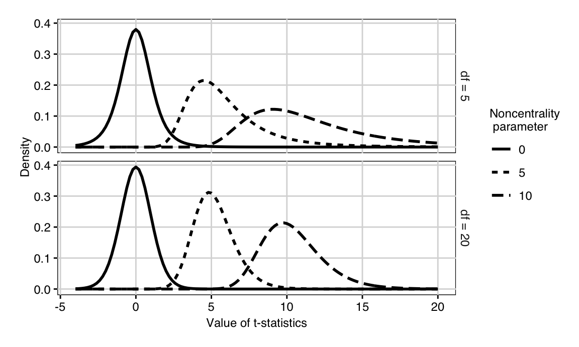
Figure 3.2: t-distribution for 5 (top) and 20 (bottom) degrees of freedom and three different noncentrality parameters (linetype).

An increase in sample size has two effects on the distribution of the test statistic \(T\): (i) it moves the critical values inwards, although this effect is only pronounced for small sample sizes; (ii) it increases the noncentrality parameter with \(\sqrt{n}\) and thereby shifts the distribution away from zero. This is in contrast to our earlier discussion using a normal distribution, where an increase in sample size results in a decrease in the variance.

In other words, increasing the sample size slightly alters the shape of the distribution of our test statistic, but more importantly moves it away from the central \(t\)-distribution under the null hypothesis. The overlap between the two distributions then decreases and the same observed difference between the two treatment means is more easily distinguished from a zero difference.

As an example, assume we have reason to believe that the two kits indeed give consistently different readouts. For a significance level of \(\alpha=5\%\) and \(n=\) 10, we calculate the power that we successfully detect a true difference of \(|\Delta|=\delta_0=2\), of \(\delta_0=1\), and of \(\delta_0=0.5\). Under the null hypothesis, the test statistics \(T\) has a (central) \(t\)-distribution with \(2n-2\) degrees of freedom, and we reject the hypothesis if \(|T|>t_{1-\alpha/2,\,2n-2}\) (Fig. 3.3 (top)). If however, \(\Delta=\delta_0\) is true, then the distribution of \(T\) changes to a noncentral \(t\)-distribution with \(2n-2\) degrees of freedom and noncentrality parameter \(\eta=\delta_0 / \text{se}(\hat{\Delta})\) (Fig. 3.3 (bottom)). The power \(1-\beta\) is the probability that this \(T\) falls into the rejection region and either stays above \(t_{1-\alpha/2,\,2n-2}\) or below \(t_{\alpha/2,\,2n-2}\).

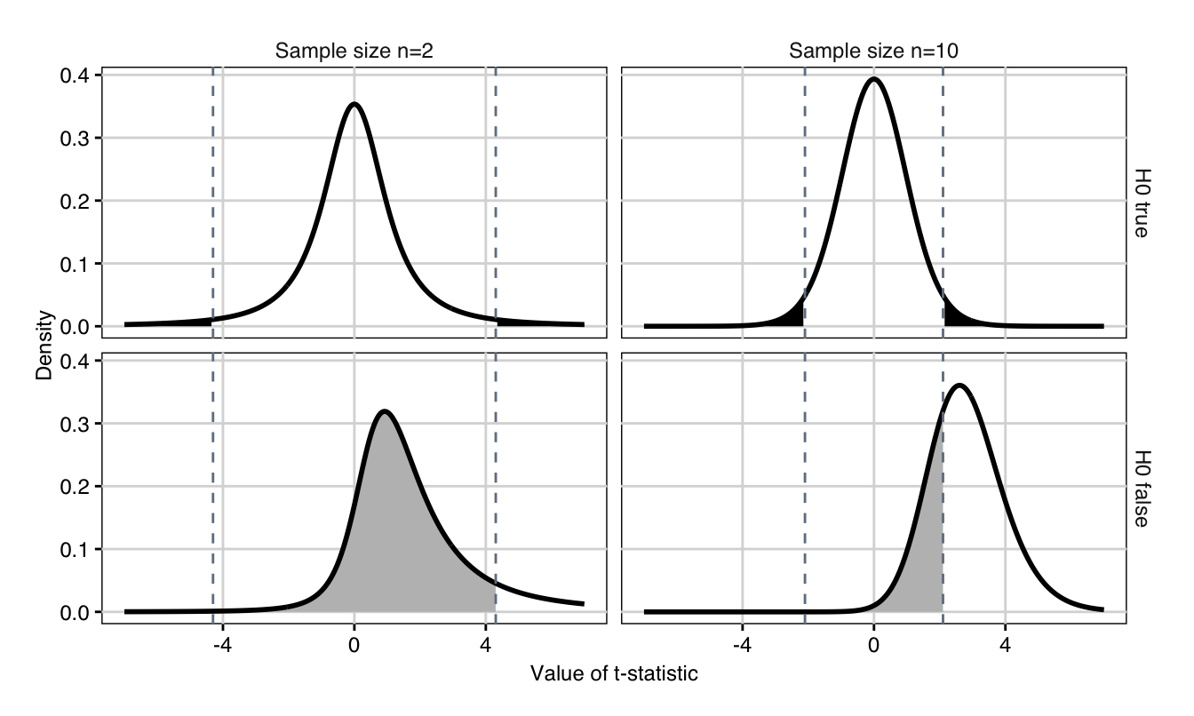
Figure 3.3: Distributions of \(t\)-statistic if null hypothesis is true and true difference is zero (top) and when alternative hypothesis is true and true difference is \(\delta_0=2\) (bottom) for 2 (left) and 10 (right) samples. The dashed lines are the critical values for the test statistic. Shaded black region: false positives (\(\alpha\)). Shaded grey region: false negatives \(\beta\).

We compute the upper \(t\)-quantile for \(n=\) 10 as \(t_{0.975,18}=\) 2.1. If the true difference is \(\delta_0=2\), then the probability to stay above this value (and correctly reject \(H_0\)) is high with a power of 73%. This is because the standard error is 0.74 and thus the precision of the estimate \(\hat{\Delta}\) is large compared to the difference we attempt to detect. Decreasing this difference while keeping the significance level and the sample size fix decreases the power to 25% for \(\delta_0=1\) and further to 10% for \(\delta_0=0.5\). In other words, we can expect to detect a true difference of \(\delta_0=0.5\) in only 10% of experiments with 10 samples per vendor and it is questionable if such an experiment is worth implementing.

It is not possible to find a closed formula for the sample size calculation, because the central and noncentral \(t\)-quantiles depend on \(n\), while the noncentrality parameter depends on \(n\) and additionally alters the shape of the noncentral \(t\)-distribution. R’s built-in function power.t.test() uses an iterative approach and yields a (deceptively precise!) sample size of \(n=\) 43.8549046 per vendor to detect a difference \(\delta_0=1\) with 80% power at a 5% significance level, based on our previous estimate \(\hat{\sigma}^2=\) 2.73 of the variance. We provide an iterative algorithm for illustration in Section 3.6.

Note that we replaced the unknown true variance with an estimate \(\hat{\sigma}^2\) for this calculation, and the accuracy of the resulting sample size hinges partly on the assumption that the variance estimate is reasonably close to the true variance.

3.5.3 Power Analysis in Practice

Power calculations are predicated on multiple assumptions such as normally distributed response values and independence of observations, all of which might hold only approximately. They also require a value for the residual variance, which is usually not known before the experiment.

In practice, we therefore base our calculations on an educated guess of this variance, or on an estimate from a previous experiment. The residual variance can sometimes be estimated from a pilot experiment, conducted to ‘test-run’ the experimental conditions and protocols of the anticipated experiment on a smaller scale. Alternatively, small experiments with a single treatment group (usually the control group) can also provide an estimate, as can perusal of previous experiments with similar experimental material.

Even though methods like power.t.test() return the sample size \(n\) with deceptively precise six decimals, it is prudent to consider the uncertainty in the variance estimate and its impact on the resulting power and sample size and to allow for a margin of error.

A very conservative approach is to consider a worst-case scenario and use the upper confidence limit instead of the variance estimate for the power analysis. In our example, we have a variance estimate of \(\hat{\sigma}^2=\) 2.73. The 95%-confidence interval of this estimate is [1.56, 5.97] and is based on \(2n-2=\) 18 degrees of freedom. For a desired power of 80% and a significance level of 5%, we found that we need 44 mice per group for detecting a difference of \(\delta_0=\) 1 based on the point estimate for \(\sigma^2\). If we use the upper confidence limit instead, the sample size increases by \(\text{UCL}/\hat{\sigma}^2\approx\) 5.97 / 2.73 = 2.2 to \(n=\) 95.

A more optimistic approach uses the estimated variance for the calculation and then adds a safety margin to the resulting sample size to compensate for uncertainties. The margin is fully at the discretion of the researcher, but adding 20%–30% to the sample size seems to be reasonable in many cases. This increases the sample size in our example from 44 to 53 for a 20% margin, and to 57 for a 30% margin.

3.5.4 ‘Observed Power’ and Related Fallacies

When confronted with an undesired non-significant test outcome from their experiment, researchers sometimes calculate the observed power or retrospective power based on the effect size and residual variance estimated from the data. It is then argued that large observed power provides evidence in favor of the null hypothesis. Appealing as this idea might seem, it is fundamentally flawed and based on improper use of the concept of power.

To see this, let us imagine that two \(t\)-tests are performed, with resulting test statistics \(t_1\) and \(t_2\), and associated non-significant \(p\)-values \(p_1>\alpha\) and \(p_2>\alpha\). Assume that \(t_1>t_2\) and the first hypothesis test indicates a larger deviation from the null hypothesis. The first \(p\)-value is then smaller than the second, which we interpret as stronger—yet not significant—evidence against the null hypothesis in the first test. If we now calculate the observed power at \(t_1\), respectively \(t_2\), for our desired significance level \(\alpha\), we find that this power is larger for the first experiment since \(t_1\) is further away from the zero value. The proposed argument then claims that this larger observed power provides more evidence in favor of the null hypothesis. This directly contradicts our previous interpretation of the two \(p\)-values.

The fallacy arises because \(p\)-value and observed power are both based on the same (random) values of the test statistic and residual variance estimated from the specific data of each experiment. This always results in higher observed power for lower \(p\)-values and leads to the apparent contradiction in the example. Indeed, it can be shown that the observed power is in direct correspondence to the \(p\)-value and therefore provides no additional information.

Similar problems result if the power is based on the observed residual variance, but calculated at a specific effect size deemed scientifically relevant. Because it is again based on the specific outcome of the experiment, this power cannot be interpreted as the power to detect an effect of the specific size and provides no evidence in favor or against the null hypothesis.

We have already seen a much better—and logically correct—way of interpreting a (non-significant) test result by estimating the difference and calculating its confidence interval. In contrast to observed power, \(p\)-value and confidence interval provide different pieces of information and there is no direct correspondence between. If the interval is wide and contains the value zero, as in our unpaired vendor example, we conclude that the data provide little evidence for or against the null hypothesis. If the interval is short, as in our paired vendor example, we conclude that plausible values are restricted to a narrow range. If this range includes zero, we have evidence that the true value is unlikely to be far off zero.

An equivalent argument can be made using two one-sided significance tests, where the null hypotheses are \(H_0:\Delta<-\delta_0\) and \(H_0:\Delta>+\delta_0\). Note that these reverse the burden of proof and a rejection of both hypotheses means that the true difference is likely in the interval \((-\delta_0,+\delta_0)\). This is known as an equivalence test, where the aim is to show that two treatments are equal (rather than different). These tests play a prominent role in toxicity or environmental studies, where we try to demonstrate that responses from a treatment group exposed to a potential hazard are no different than \(\pm\delta_0\) compared to a non-exposed group.

Calculating power prospectively in the planning of an experiment ensures that tests are adequately powered and estimates are sufficiently precise. Power analysis has no role retrospectively in the analysis of data from an experiment. Here, estimates of effect sizes and their confidence intervals are the appropriate quantities, augmented by \(p\)-values if necessary.

3.6 Notes and Summary

Notes

A general discussion of power and sample size is given in Cohen (1988), Cohen (1992), and Krzywinski and Altman (2013), and a gentle practical introduction is Lenth (2001). Sample sizes for confidence intervals are addressed in Goodman and Berlin (1994), Maxwell, Kelley, and Rausch (2008), and Rothman and Greenland (2018); the equivalence to power calculation based on testing is discussed in Altman et al. (2000). The fallacies of ‘observed power’ are elucidated in Hoenig and Heisey (2001), and equivalence testing in Schuirmann (1987). The free software G*Power is an alternative to R for sample size determination (Faul et al. 2007).

Power analysis code

To further illustrate our power analysis, we implement the corresponding calculations in an R function. The following code calculates the power of a \(t\)-test given the minimal difference delta, the significance level alpha, the sample size n, and the standard deviation s.

The function first calculates the degrees of freedom for the given sample size. Then, the lower and upper critical values for the \(t\)-statistic under the null hypothesis are computed. Next, the noncentrality parameter \(\eta=\) ncp is used to determine the probability of correctly rejecting \(H_0\) if indeed \(|\Delta|=\delta_0\); this is precisely the power.

We start from a reasonably low \(n\), calculate the power, and increase the sample size until the desired power is reached.

# delta0: true difference
# alpha: significance level (false positive rate)
# n: sample size
# s: standard deviation
# return: power
getPowerT = function(delta0, alpha, n, s) {
  df = 2*n-2  # degrees of freedom
  q.H0.low = qt(p=alpha/2, df=df)    # low rejection quantile
  q.H0.high = qt(p=1-alpha/2, df=df) # high rejection quantile
  ncp = abs(delta0) / (sqrt(2)*s/sqrt(n)) # noncentrality
  # prob. to reject low or high values if H0 false
  p.low = pt(q=q.H0.low, df=df, ncp=ncp)
  p.high = 1 - pt(q=q.H0.high, df=df, ncp=ncp)
  return( p.low + p.high )
}

Using R

Base-R provides the power.t.test() function for power calculations based on the \(t\)-distribution. It takes four of the five parameters and calculates the fifth.

Summary

Determining the required sample size of an experiment—at least approximately—is part of the experimental design. We can use the hypothesis testing framework to determine sample size based on the two error probabilities, a measure of variation, and the required minimal effect size. The resulting sample size should then be used to determine if estimates have sufficient expected precision. We can also determine the minimal effect size detectable with desired power and sample size, or the power achieved from a given sample size for a minimal effect size, all of which we can use to decide if an experiment is worth doing. Precision and power can also be increased without increasing the sample size, by balanced allocation, narrowing experimental conditions, or blocking. Power analysis is often based on noncentral distributions, whose noncentrality parameters are the product of experiment size and effect size; portable power formulas use approximations of various quantities to allow back-of-envelope power analysis.