Chapter 1 Principles of Experimental Design
1.1 Introduction
The validity of conclusions drawn from a statistical analysis crucially hinges on the manner in which the data are acquired, and even the most sophisticated analysis will not rescue a flawed experiment. Planning an experiment and thinking about the details of data acquisition is so important for a successful analysis that R. A. Fisher—who single-handedly invented many of the experimental design techniques we are about to discuss—famously wrote
To call in the statistician after the experiment is done may be no more than asking him to perform a post-mortem examination: he may be able to say what the experiment died of. (Fisher 1938)
(Statistical) design of experiments provides the principles and methods for planning experiments and tailoring the data acquisition to an intended analysis. Design and analysis of an experiment are best considered as two aspects of the same enterprise: the goals of the analysis strongly inform an appropriate design, and the implemented design determines the possible analyses.
The primary aim of designing experiments is to ensure that valid statistical and scientific conclusions can be drawn that withstand the scrutiny of a determined skeptic. Good experimental design also considers that resources are used efficiently, and that estimates are sufficiently precise and hypothesis tests adequately powered. It protects our conclusions by excluding alternative interpretations or rendering them implausible. Three main pillars of experimental design are randomization, replication, and blocking, and we will flesh out their effects on the subsequent analysis as well as their implementation in an experimental design.
An experimental design is always tailored towards predefined (primary) analyses and an efficient analysis and unambiguous interpretation of the experimental data is often straightforward from a good design. This does not prevent us from doing additional analyses of interesting observations after the data are acquired, but these analyses can be subjected to more severe criticisms and conclusions are more tentative.
In this chapter, we provide the wider context for using experiments in a larger research enterprise and informally introduce the main statistical ideas of experimental design. We use a comparison of two samples as our main example to study how design choices affect an analysis, but postpone a formal quantitative analysis to the next chapters.
1.2 A Cautionary Tale
For illustrating some of the issues arising in the interplay of experimental design and analysis, we consider a simple example. We are interested in comparing the enzyme levels measured in processed blood samples from laboratory mice, when the sample processing is done either with a kit from a vendor A, or a kit from a competitor B. For this, we take 20 mice and randomly select 10 of them for sample preparation with kit A, while the blood samples of the remaining 10 mice are prepared with kit B. The experiment is illustrated in Figure 1.1A and the resulting data are given in Table 1.1.
| A | 8.96 | 8.95 | 11.37 | 12.63 | 11.38 | 8.36 | 6.87 | 12.35 | 10.32 | 11.99 |
| B | 12.68 | 11.37 | 12.00 | 9.81 | 10.35 | 11.76 | 9.01 | 10.83 | 8.76 | 9.99 |
One option for comparing the two kits is to look at the difference in average enzyme levels, and we find an average level of 10.32 for vendor A and 10.66 for vendor B. We would like to interpret their difference of -0.34 as the difference due to the two preparation kits and conclude whether the two kits give equal results or if measurements based on one kit are systematically different from those based on the other kit.
Such interpretation, however, is only valid if the two groups of mice and their measurements are identical in all aspects except the sample preparation kit. If we use one strain of mice for kit A and another strain for kit B, any difference might also be attributed to inherent differences between the strains. Similarly, if the measurements using kit B were conducted much later than those using kit A, any observed difference might be attributed to changes in, e.g., mice selected, batches of chemicals used, device calibration, or any number of other influences. None of these competing explanations for an observed difference can be excluded from the given data alone, but good experimental design allows us to render them (almost) arbitrarily implausible.
A second aspect for our analysis is the inherent uncertainty in our calculated difference: if we repeat the experiment, the observed difference will change each time, and this will be more pronounced for a smaller number of mice, among others. If we do not use a sufficient number of mice in our experiment, the uncertainty associated with the observed difference might be too large, such that random fluctuations become a plausible explanation for the observed difference. Systematic differences between the two kits, of practically relevant magnitude in either direction, might then be compatible with the data, and we can draw no reliable conclusions from our experiment.
In each case, the statistical analysis—no matter how clever—was doomed before the experiment was even started, while simple ideas from statistical design of experiments would have provided correct and robust results with interpretable conclusions.
1.3 The Language of Experimental Design
By an experiment we understand an investigation where the researcher has full control over selecting and altering the experimental conditions of interest, and we only consider investigations of this type. The selected experimental conditions are called treatments. An experiment is comparative if the responses to several treatments are to be compared or contrasted. The experimental units are the smallest subdivision of the experimental material to which a treatment can be assigned. All experimental units given the same treatment constitute a treatment group. Especially in biology, we often compare treatments to a control group to which some standard experimental conditions are applied; a typical example is using a placebo for the control group, and different drugs for the other treatment groups.
The values observed are called responses and are measured on the response units; these are often identical to the experimental units but need not be. Multiple experimental units are sometimes combined into groupings or blocks, such as mice grouped by litter, or samples grouped by batches of chemicals used for their preparation. More generally, we call any grouping of the experimental material (even with group size one) a unit.
In our example, we selected the mice, used a single sample per mouse, deliberately chose the two specific vendors, and had full control over which kit to assign to which mouse. In other words, the two kits are the treatments and the mice are the experimental units. We took the measured enzyme level of a single sample from a mouse as our response, and samples are therefore the response units. The resulting experiment is comparative, because we contrast the enzyme levels between the two treatment groups.
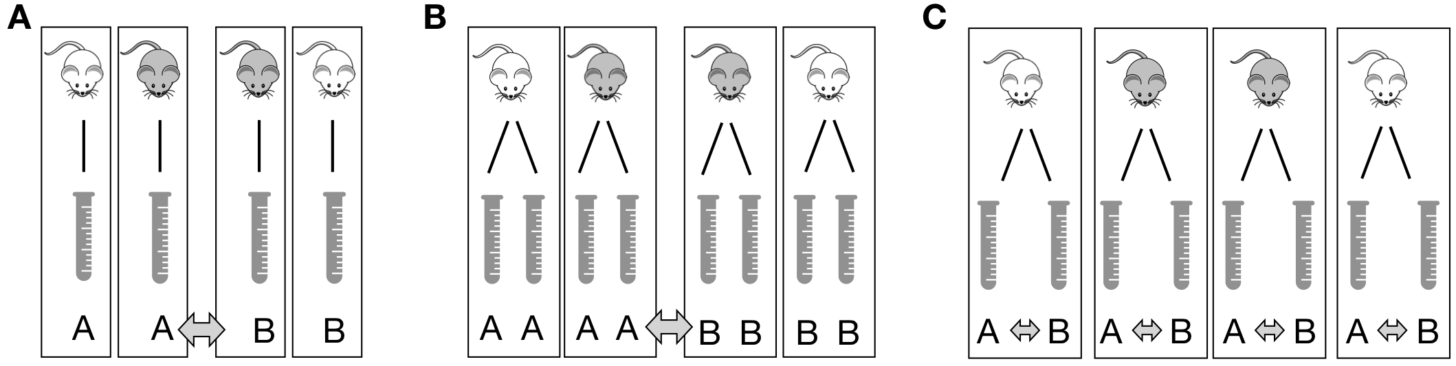
Figure 1.1: Three designs to determine the difference between two preparation kits A and B based on four mice. A: One sample per mouse. Comparison between averages of samples with same kit. B: Two samples per mouse treated with the same kit. Comparison between averages of mice with same kit requires averaging responses for each mouse first. C: Two samples per mouse each treated with different kit. Comparison between two samples of each mouse, with differences averaged.
In this example, we can coalesce experimental and response units, because we have a single response per mouse and cannot distinguish a sample from a mouse in the analysis, as illustrated in Figure 1.1A for four mice. Responses from mice with the same kit are averaged, and the kit difference is the difference between these two averages.
By contrast, if we take two samples per mouse and use the same kit for both samples, then the mice are still the experimental units, but each mouse now groups the two response units associated with it. Now, responses from the same mouse are first averaged, and these averages are used to calculate the difference between kits; even though eight measurements are available, this difference is still based on only four mice (Figure 1.1B).
If we take two samples per mouse, but apply each kit to one of the two samples, then the samples are both the experimental and response units, while the mice are blocks that group the samples. Now, we calculate the difference between kits for each mouse, and then average these differences (Figure 1.1C).
If we only use one kit and determine the average enzyme level, then this investigation is still an experiment, but is not comparative.
To summarize, the design of an experiment determines the logical structure of the experiment; it consists of (i) a set of treatments (the two kits); (ii) a specification of the experimental units (animals, cell lines, samples) (the mice in Figure 1.1A,B and the samples in Figure 1.1C); (iii) a procedure for assigning treatments to units; and (iv) a specification of the response units and the quantity to be measured as a response (the samples and associated enzyme levels).
1.4 Experiment Validity
Before we embark on the more technical aspects of experimental design, we discuss three components for evaluating an experiment’s validity: construct validity, internal validity, and external validity. These criteria are well-established in areas such as educational and psychological research, and have more recently been discussed for animal research (Würbel 2017) where experiments are increasingly scrutinized for their scientific rationale and their design and intended analyses.
1.4.1 Construct Validity
Construct validity concerns the choice of the experimental system for answering our research question. Is the system even capable of providing a relevant answer to the question?
Studying the mechanisms of a particular disease, for example, might require careful choice of an appropriate animal model that shows a disease phenotype and is accessible to experimental interventions. If the animal model is a proxy for drug development for humans, biological mechanisms must be sufficiently similar between animal and human physiologies.
Another important aspect of the construct is the quantity that we intend to measure (the measurand), and its relation to the quantity or property we are interested in. For example, we might measure the concentration of the same chemical compound once in a blood sample and once in a highly purified sample, and these constitute two different measurands, whose values might not be comparable. Often, the quantity of interest (e.g., liver function) is not directly measurable (or even quantifiable) and we measure a biomarker instead. For example, pre-clinical and clinical investigations may use concentrations of proteins or counts of specific cell types from blood samples, such as the CD4+ cell count used as a biomarker for immune system function.
1.4.2 Internal Validity
The internal validity of an experiment concerns the soundness of the scientific rationale, statistical properties such as precision of estimates, and the measures taken against risk of bias. It refers to the validity of claims within the context of the experiment. Statistical design of experiments plays a prominent role in ensuring internal validity, and we briefly discuss the main ideas before providing the technical details and an application to our example in the subsequent sections.
Scientific Rationale and Research Question
The scientific rationale of a study is (usually) not immediately a statistical question. Translating a scientific question into a quantitative comparison amenable to statistical analysis is no small task and often requires careful consideration. It is a substantial, if non-statistical, benefit of using experimental design that we are forced to formulate a precise-enough research question and decide on the main analyses required for answering it before we conduct the experiment. For example, the question: is there a difference between placebo and drug? is insufficiently precise for planning a statistical analysis and determine an adequate experimental design. What exactly is the drug treatment? What should the drug’s concentration be and how is it administered? How do we make sure that the placebo group is comparable to the drug group in all other aspects? What do we measure and what do we mean by “difference?” A shift in average response, a fold-change, change in response before and after treatment?
The scientific rationale also enters the choice of a potential control group to which we compare responses. The quote
The deep, fundamental question in statistical analysis is ‘Compared to what?’ (Tufte 1997)
highlights the importance of this choice.
There are almost never enough resources to answer all relevant scientific questions. We therefore define a few questions of highest interest, and the main purpose of the experiment is answering these questions in the primary analysis. This intended analysis drives the experimental design to ensure relevant estimates can be calculated and have sufficient precision, and tests are adequately powered. This does not preclude us from conducting additional secondary analyses and exploratory analyses, but we are not willing to enlarge the experiment to ensure that strong conclusions can also be drawn from these analyses.
Risk of Bias
Experimental bias is a systematic difference in response between experimental units in addition to the difference caused by the treatments. The experimental units in the different groups are then not equal in all aspects other than the treatment applied to them. We saw several examples in Section 1.2.
Minimizing the risk of bias is crucial for internal validity and we look at some common measures to eliminate or reduce different types of bias in Section 1.5.
Precision and Effect Size
Another aspect of internal validity is the precision of estimates and the expected effect sizes. Is the experimental setup, in principle, able to detect a difference of relevant magnitude? Experimental design offers several methods for answering this question based on the expected heterogeneity of samples, the measurement error, and other sources of variation: power analysis is a technique for determining the number of samples required to reliably detect a relevant effect size and provide estimates of sufficient precision. More samples yield more precision and more power, but we have to be careful that replication is done at the right level: simply measuring a biological sample multiple times as in Figure 1.1B yields more measured values, but is pseudo-replication for analyses. Replication should also ensure that the statistical uncertainties of estimates can be gauged from the data of the experiment itself, without additional untestable assumptions. Finally, the technique of blocking, shown in Figure 1.1C, can remove a substantial proportion of the variation and thereby increase power and precision if we find a way to apply it.
1.4.3 External Validity
The external validity of an experiment concerns its replicability and the generalizability of inferences. An experiment is replicable if its results can be confirmed by an independent new experiment, preferably by a different lab and researcher. Experimental conditions in the replicate experiment usually differ from the original experiment, which provides evidence that the observed effects are robust to such changes. A much weaker condition on an experiment is reproducibility, the property that an independent researcher draws equivalent conclusions based on the data from this particular experiment, using the same analysis techniques. Reproducibility requires publishing the raw data, details on the experimental protocol, and a description of the statistical analyses, preferably with accompanying source code. Many scientific journals subscribe to reporting guidelines to ensure reproducibility and these are also helpful for planning an experiment.
A main threat to replicability and generalizability are too tightly controlled experimental conditions, when inferences only hold for a specific lab under the very specific conditions of the original experiment. Introducing systematic heterogeneity and using multi-center studies effectively broadens the experimental conditions and therefore the inferences for which internal validity is available.
For systematic heterogeneity, experimental conditions are systematically altered in addition to the treatments, and treatment differences estimated for each condition. For example, we might split the experimental material into several batches and use a different day of analysis, sample preparation, batch of buffer, measurement device, and lab technician for each batch. A more general inference is then possible if effect size, effect direction, and precision are comparable between the batches, indicating that the treatment differences are stable over the different conditions.
In multi-center experiments, the same experiment is conducted in several different labs and the results compared and merged. Multi-center approaches are very common in clinical trials and often necessary to reach the required number of patient enrollments.
Generalizability of randomized controlled trials in medicine and animal studies can suffer from overly restrictive eligibility criteria. In clinical trials, patients are often included or excluded based on co-medications and co-morbidities, and the resulting sample of eligible patients might no longer be representative of the patient population. For example, Travers et al. (2007) used the eligibility criteria of 17 random controlled trials of asthma treatments and found that out of 749 patients, only a median of 6% (45 patients) would be eligible for an asthma-related randomized controlled trial. This puts a question mark on the relevance of the trials’ findings for asthma patients in general.
1.5 Reducing the Risk of Bias
1.5.1 Randomization of Treatment Allocation
If systematic differences other than the treatment exist between our treatment groups, then the effect of the treatment is confounded with these other differences and our estimates of treatment effects might be biased.
We remove such unwanted systematic differences from our treatment comparisons by randomizing the allocation of treatments to experimental units. In a completely randomized design, each experimental unit has the same chance of being subjected to any of the treatments, and any differences between the experimental units other than the treatments are distributed over the treatment groups. Importantly, randomization is the only method that also protects our experiment against unknown sources of bias: we do not need to know all or even any of the potential differences and yet their impact is eliminated from the treatment comparisons by random treatment allocation.
Randomization has two effects: (i) differences unrelated to treatment become part of the ‘statistical noise’ rendering the treatment groups more similar; and (ii) the systematic differences are thereby eliminated as sources of bias from the treatment comparison.
Randomization transforms systematic variation into random variation.
In our example, a proper randomization would select 10 out of our 20 mice fully at random, such that the probability of any one mouse being picked is 1/20. These ten mice are then assigned to kit A, and the remaining mice to kit B. This allocation is entirely independent of the treatments and of any properties of the mice.
To ensure random treatment allocation, some kind of random process needs to be employed. This can be as simple as shuffling a pack of 10 red and 10 black cards or using a software-based random number generator. Randomization is slightly more difficult if the number of experimental units is not known at the start of the experiment, such as when patients are recruited for an ongoing clinical trial (sometimes called rolling recruitment), and we want to have reasonable balance between the treatment groups at each stage of the trial.
Seemingly random assignments “by hand” are usually no less complicated than fully random assignments, but are always inferior. If surprising results ensue from the experiment, such assignments are subject to unanswerable criticism and suspicion of unwanted bias. Even worse are systematic allocations; they can only remove bias from known causes, and immediately raise red flags under the slightest scrutiny.
The Problem of Undesired Assignments
Even with a fully random treatment allocation procedure, we might end up with an undesirable allocation. For our example, the treatment group of kit A might—just by chance—contain mice that are all bigger or more active than those in the other treatment group. Statistical orthodoxy recommends using the design nevertheless, because only full randomization guarantees valid estimates of residual variance and unbiased estimates of effects. This argument, however, concerns the long-run properties of the procedure and seems of little help in this specific situation. Why should we care if the randomization yields correct estimates under replication of the experiment, if the particular experiment is jeopardized?
Another solution is to create a list of all possible allocations that we would accept and randomly choose one of these allocations for our experiment. The analysis should then reflect this restriction in the possible randomizations, which often renders this approach difficult to implement.
The most pragmatic method is to reject highly undesirable designs and compute a new randomization (Cox 1958). Undesirable allocations are unlikely to arise for large sample sizes, and we might accept a small bias in estimation for small sample sizes, when uncertainty in the estimated treatment effect is already high. In this approach, whenever we reject a particular outcome, we must also be willing to reject the outcome if we permute the treatment level labels. If we reject eight big and two small mice for kit A, then we must also reject two big and eight small mice. We must also be transparent and report a rejected allocation, so that critics may come to their own conclusions about potential biases and their remedies.
1.5.2 Blinding
Bias in treatment comparisons is also introduced if treatment allocation is random, but responses cannot be measured entirely objectively, or if knowledge of the assigned treatment affects the response. In clinical trials, for example, patients might react differently when they know to be on a placebo treatment, an effect known as cognitive bias. In animal experiments, caretakers might report more abnormal behavior for animals on a more severe treatment. Cognitive bias can be eliminated by concealing the treatment allocation from technicians or participants of a clinical trial, a technique called single-blinding.
If response measures are partially based on professional judgement (such as a clinical scale), patient or physician might unconsciously report lower scores for a placebo treatment, a phenomenon known as observer bias. Its removal requires double blinding, where treatment allocations are additionally concealed from the experimentalist.
Blinding requires randomized treatment allocation to begin with and substantial effort might be needed to implement it. Drug companies, for example, have to go to great lengths to ensure that a placebo looks, tastes, and feels similar enough to the actual drug. Additionally, blinding is often done by coding the treatment conditions and samples, and effect sizes and statistical significance are calculated before the code is revealed.
In clinical trials, double-blinding creates a conflict of interest. The attending physicians do not know which patient received which treatment, and thus accumulation of side-effects cannot be linked to any treatment. For this reason, clinical trials have a data monitoring committee not involved in the final analysis, that performs intermediate analyses of efficacy and safety at predefined intervals. If severe problems are detected, the committee might recommend altering or aborting the trial. The same might happen if one treatment already shows overwhelming evidence of superiority, such that it becomes unethical to withhold this treatment from the other patients.
1.5.3 Analysis Plan and Registration
An often overlooked source of bias has been termed the researcher degrees of freedom or garden of forking paths in the data analysis. For any set of data, there are many different options for its analysis: some results might be considered outliers and discarded, assumptions are made on error distributions and appropriate test statistics, different covariates might be included into a regression model. Often, multiple hypotheses are investigated and tested, and analyses are done separately on various (overlapping) subgroups. Hypotheses formed after looking at the data require additional care in their interpretation; almost never will \(p\)-values for these ad hoc or post hoc hypotheses be statistically justifiable. Many different measured response variables invite fishing expeditions, where patterns in the data are sought without an underlying hypothesis. Only reporting those sub-analyses that gave ‘interesting’ findings invariably leads to biased conclusions and is called cherry-picking or \(p\)-hacking (or much less flattering names).
The statistical analysis is always part of a larger scientific argument and we should consider the necessary computations in relation to building our scientific argument about the interpretation of the data. In addition to the statistical calculations, this interpretation requires substantial subject-matter knowledge and includes (many) non-statistical arguments. Two quotes highlight that experiment and analysis are a means to an end and not the end in itself.
There is a boundary in data interpretation beyond which formulas and quantitative decision procedures do not go, where judgment and style enter. (Abelson 1995)
Often, perfectly reasonable people come to perfectly reasonable decisions or conclusions based on nonstatistical evidence. Statistical analysis is a tool with which we support reasoning. It is not a goal in itself. (Bailar III 1981)
There is often a grey area between exploiting researcher degrees of freedom to arrive at a desired conclusion, and creative yet informed analyses of data. One way to navigate this area is to distinguish between exploratory studies and confirmatory studies. The former have no clearly stated scientific question, but are used to generate interesting hypotheses by identifying potential associations or effects that are then further investigated. Conclusions from these studies are very tentative and must be reported honestly as such. In contrast, standards are much higher for confirmatory studies, which investigate a specific predefined scientific question. Analysis plans and pre-registration of an experiment are accepted means for demonstrating lack of bias due to researcher degrees of freedom, and separating primary from secondary analyses allows emphasizing the main goals of the study.
Analysis Plan
The analysis plan is written before conducting the experiment and details the measurands and estimands, the hypotheses to be tested together with a power and sample size calculation, a discussion of relevant effect sizes, detection and handling of outliers and missing data, as well as steps for data normalization such as transformations and baseline corrections. If a regression model is required, its factors and covariates are outlined. Particularly in biology, handling measurements below the limit of quantification and saturation effects require careful consideration.
In the context of clinical trials, the problem of estimands has become a recent focus of attention. An estimand is the target of a statistical estimation procedure, for example the true average difference in enzyme levels between the two preparation kits. A main problem in many studies are post-randomization events that can change the estimand, even if the estimation procedure remains the same. For example, if kit B fails to produce usable samples for measurement in five out of ten cases because the enzyme level was too low, while kit A could handle these enzyme levels perfectly fine, then this might severely exaggerate the observed difference between the two kits. Similar problems arise in drug trials, when some patients stop taking one of the drugs due to side-effects or other complications.
Registration
Registration of experiments is an even more severe measure used in conjunction with an analysis plan and is becoming standard in clinical trials. Here, information about the trial, including the analysis plan, procedure to recruit patients, and stopping criteria, are registered in a public database. Publications based on the trial then refer to this registration, such that reviewers and readers can compare what the researchers intended to do and what they actually did. Similar portals for pre-clinical and translational research are also available.
1.6 Notes and Summary
Notes
The problem of measurements and measurands is further discussed for statistics in Hand (1996) and specifically for biological experiments in Coxon, Longstaff, and Burns (2019). A general review of methods for handling missing data is Dong and Peng (2013). The different roles of randomization are emphasized in Cox (2009).
Two well-known reporting guidelines are the ARRIVE guidelines for animal research (Kilkenny et al. 2010) and the CONSORT guidelines for clinical trials (Moher et al. 2010). Guidelines describing the minimal information required for reproducing experimental results have been developed for many types of experimental techniques, including microarrays (MIAME), RNA sequencing (MINSEQE), metabolomics (MSI) and proteomics (MIAPE) experiments; the FAIRSHARE initiative provides a more comprehensive collection (Sansone et al. 2019).
The problems of experimental design in animal experiments and particularly translation research are discussed in Couzin-Frankel (2013). Multi-center studies are now considered for these investigations, and using a second laboratory already increases reproducibility substantially (Richter et al. 2010; Richter 2017; Voelkl et al. 2018; Karp 2018) and allows standardizing the treatment effects (Kafkafi et al. 2017). First attempts are reported of using designs similar to clinical trials (Llovera and Liesz 2016). Exploratory-confirmatory research and external validity for animal studies is discussed in Kimmelman, Mogil, and Dirnagl (2014) and Pound and Ritskes-Hoitinga (2018). Further information on pilot studies is found in Moore et al. (2011), Sim (2019), and Thabane et al. (2010).
The deliberate use of statistical analyses and their interpretation for supporting a larger argument was called statistics as principled argument (Abelson 1995). Employing useless statistical analysis without reference to the actual scientific question is surrogate science (Gigerenzer and Marewski 2014) and adaptive thinking is integral to meaningful statistical analysis (Gigerenzer 2002).
Summary
In an experiment, the investigator has full control over the experimental conditions applied to the experiment material. The experimental design gives the logical structure of an experiment: the units describing the organization of the experimental material, the treatments and their allocation to units, and the response. Statistical design of experiments includes techniques to ensure internal validity of an experiment, and methods to make inference from experimental data efficient.