Chapter 5 Comparing Treatment Groups with Linear Contrasts
5.1 Introduction
The omnibus \(F\)-test appraises the evidence against the hypothesis of identical group means, but a rejection of this null hypothesis provides little information about which groups differ and how. A very general and elegant framework for evaluating treatment group differences are linear contrasts, which provide a principled way for constructing corresponding \(t\)-tests and confidence intervals. In this chapter, we develop this framework and apply it to our four drugs example; we also consider several more complex examples to demonstrate its power and versatility.
If a set of contrasts is orthogonal, then we can reconstitute the result of the \(F\)-test using the results from the contrasts, and a significant \(F\)-test implies that at least one contrast is significant. If the \(F\)-test is not significant, we might still find significant contrasts, because the \(F\)-test considers all deviations from equal group means simultaneously, while a contrast looks for a specific set of deviations for which it provides more power by ignoring other potential deviations.
Considering several contrasts leads to a multiplicity problem that requires adjusting confidence and significance levels. Several multiple comparison procedures allow us to calculate these adjustments for different sets of contrasts.
5.2 Linear Contrasts
For our example, we might be interested in comparing the two drugs \(D1\) and \(D2\), for example. One way of doing this is by a simple \(t\)-test between the corresponding observations. This yields a \(t\)-value of \(t=\) 2.22 and a \(p\)-value of \(p=\) 0.044 for a difference of \(\hat{\mu}_1-\hat{\mu}_2=\) 1.52 with a 95%-confidence interval [0.05, 2.98]. While this approach yields a valid estimate and test, it is inefficient because we completely neglect the information available in the observations of drugs \(D3\) and \(D4\). Specifically, if we assume that the variances are the same in all treatment groups, we could use these additional observations to get a better estimate of the residual variance \(\sigma_e^2\) and increase the degrees of freedom.
We consider three example comparisons using our four drugs. We additionally assume that \(D1\) and \(D2\) share the same active component and denote these drugs as “Class A,” while \(D3\) and \(D4\) share another component (“Class B”):
- as before, compare the drugs in the first class: \(D1\) versus \(D2\);
- compare the drugs in the second class: \(D3\) versus \(D4\);
- compare the classes: average of \(D1\) and \(D2\) versus average of \(D3\) and \(D4\).
We can formulate these comparisons in terms of differences of treatment group means; each is an example of a linear contrast: \[\begin{align*} \text{D1 vs D2} &: \mu_1-\mu_2 \\ \text{D3 vs D4} &: \mu_3-\mu_4 \\ \text{Class A vs Class B} &: \left(\frac{\mu_1+\mu_2}{2}\right)-\left(\frac{\mu_3+\mu_4}{2}\right)\;. \end{align*}\] Note that a \(t\)-test for the third comparison requires manual calculation of the corresponding estimates and their standard errors first.
Linear contrasts use all data for estimation and ‘automatically’ lead to the correct \(t\)-test and confidence interval calculations. Their estimation is one of the main purposes for an experiment:
Contrasts of interest justify the design, not the other way around.
An important task in designing an experiment is to ensure that contrasts of interest are defined beforehand and can be estimated with adequate precision.
5.2.1 Defining Contrasts
Formally, a linear contrast \(\Psi(\mathbf{w})\) for a treatment factor with \(k\) levels is a linear combination of the group means using a weight vector \(\mathbf{w}=(w_1,\dots,w_k)\): \[ \Psi(\mathbf{w}) = w_1\cdot\mu_1 + \cdots + w_k\cdot\mu_k \;, \] where the entries in the weight vector sum to zero, such that \(w_1+\cdots +w_k=0\).
We compare the group means of two sets \(X\) and \(Y\) of treatment factor levels by selecting the weights \(w_i\) as follows:
- the weight of each treatment level not considered is zero: \(w_i=0\iff i\not\in X\) and \(i\not\in Y\);
- the weights for set \(X\) are all positive: \(w_i>0\iff i\in X\);
- the weights for set \(Y\) are all negative: \(w_i<0\iff i\in Y\);
- the weights sum to zero: \(w_1+\cdots +w_k=0\);
- the individual weights \(w_i\) determine how the group means of the sets \(X\) and \(Y\) are averaged; using equal weights with each set corresponds to a simple average of the set’s group means.
The weight vectors for our example contrasts are \(\mathbf{w}_1=(+1,-1,0,0)\) for the first contrast, where \(X=\{1\}\) and \(Y=\{2\}\); \(\mathbf{w}_2=(0,0,+1,-1)\) for the second, \(X=\{3\}\) and \(Y=\{4\}\); and \(\mathbf{w}_3=(+1/2, +1/2, -1/2, -1/2)\) for the third contrast, where \(X=\{1,2\}\) and \(Y=\{3,4\}\).
5.2.2 Estimating Contrasts
We estimate a contrast by replacing the group means by their estimates: \[ \hat{\Psi}(\mathbf{w}) = w_1\cdot\hat{\mu}_1 + \cdots + w_k\cdot\hat{\mu}_k \;. \] Unbalancedness only affects the precision but not the interpretation of contrast estimates, and we can make our exposition more general by allowing different numbers of samples per group, denoting by \(n_i\) the number of samples in group \(i\). From the properties of the group mean estimates \(\hat{\mu}_i\), we know that \(\hat{\Psi}(\mathbf{w})\) is an unbiased estimator of the contrast \(\Psi(\mathbf{w})\) and has variance \[ \text{Var}\left(\hat{\Psi}(\mathbf{w})\right) = \text{Var}\left(w_1\cdot\hat{\mu}_1 + \cdots + w_k\cdot\hat{\mu}_k\right) = \sum_{i=1}^k w_i^2 \cdot\text{Var}(\hat{\mu}_i) = \sigma_e^2\cdot\sum_{i=1}^k \frac{w_i^2}{n_i}\;. \] We can thus estimate its standard error by \[ \widehat{\text{se}}\left(\hat{\Psi}(\mathbf{w})\right) = \hat{\sigma}_e\cdot\sqrt{\sum_{i=1}^k\frac{w_i^2}{n_i}}\;. \] Note that the precision of a contrast estimate depends on the sizes for the involved groups (i.e., those with \(w_i\not= 0\)) in an unbalanced design, and standard errors are higher for contrasts involving groups with low numbers of replicates in this case.
The estimate of a contrast is based on the normally distributed estimates of the group means. We can use the residual variance estimate from the preceding ANOVA, and the resulting estimator for any contrast has a \(t\)-distribution with all \(N-k\) degrees of freedom.
This immediately yields a \((1-\alpha)\)-confidence interval for a contrast estimate \(\hat{\Psi}(\mathbf{w})\): \[ \hat{\Psi}(\mathbf{w}) \pm t_{\alpha/2, N-k}\cdot \widehat{\text{se}}\left(\hat{\Psi}(\mathbf{w})\right) = \hat{\Psi}(\mathbf{w}) \pm t_{\alpha/2, N-k}\cdot\hat{\sigma}_e\cdot\sqrt{\sum_{i=1}^k\frac{w_i^2}{n_i}}\;, \] where again \(t_{\alpha/2, N-k}\) is the \(\alpha/2\)-quantile of the \(t\)-distribution with \(N-k\) degrees of freedom (\(N\) the total number of samples). If the degrees of freedom are sufficiently large, we can alternatively calculate the confidence interval based on the normal quantiles by replacing the quantile \(t_{\alpha/2, N-k}\) with \(z_{\alpha/2}\).
For our third example contrast, we find an estimate of \(\hat{\Psi}(\mathbf{w}_3)=\) 4.28 for the difference between the average enzyme levels for a class A and class B drug. We already have an estimate \(\hat{\sigma}_e=\) 1.22 of the residual standard deviation: it is the root of the residual mean squares. The standard error of \(\hat{\Psi}(\mathbf{w}_3)\) is given by \[ \widehat{\text{se}}(\hat{\Psi}(\mathbf{w}_3)) = \hat{\sigma}_e\cdot\sqrt{\left(\frac{(0.5)^2}{8}+\frac{(0.5)^2}{8}+\frac{(-0.5)^2}{8}+\frac{(-0.5)^2}{8}\right)}\approx 0.35\cdot\hat{\sigma}_e\;, \] which yields an estimated standard error of \(\widehat{\text{se}}(\hat{\Psi}(\mathbf{w}_3))=\,\) 0.43.
From this, we calculate a \(t\)-based 95%-confidence interval of [3.4, 5.16], based on the \(t\)-quantile \(t_{0.025,28}=\) \(-2.05\) for \(N-k=\) 28 degrees of freedom. The confidence interval only contains positive values and we can therefore conclude that drugs in class A have indeed a higher enzyme level than those in class B and the observed difference between the classes is not likely due to random fluctuations in the data.
| Comparison | Contrast | Estimate | LCL | UCL |
|---|---|---|---|---|
| \(D1\)-vs-\(D2\) | \(\Psi(\mathbf{w}_1)=\mu_1-\mu_2\) | 1.51 | 0.27 | 2.76 |
| \(D3\)-vs-\(D4\) | \(\Psi(\mathbf{w}_2)=\mu_3-\mu_4\) | \(-0.1\) | \(-1.34\) | 1.15 |
| Class A-vs-Class B | \(\Psi(\mathbf{w}_3)=\frac{\mu_1+\mu_2}{2}-\frac{\mu_3+\mu_4}{2}\) | 4.28 | 3.4 | 5.16 |
Equivalent calculations for the remaining two example contrasts \(\Psi(\mathbf{w}_1)\) and \(\Psi(\mathbf{w}_2)\) yield the estimates and 95%-confidence intervals in Table 5.1. The results suggest that the two drugs \(D1\) and \(D2\) in class A lead to different enzyme levels, if only slightly so. Note that the estimate for this contrast is identical to our \(t\)-test result, but the confidence interval is substantially narrower; this is the result of pooling the data for estimating the residual variance and increasing the degrees of freedom. The two drugs in class B cannot be distinguished based on the data.
5.2.3 Testing Contrasts
A linear contrast estimate has a \(t\)-distribution for normally distributed response values. This allows us to derive a \(t\)-test for testing the null hypothesis \[ H_0: \Psi(\mathbf{w}) = 0 \] using the test statistic \[ T = \frac{\hat{\Psi}(\mathbf{w})}{\widehat{\text{se}}(\hat{\Psi}(\mathbf{w}))} = \frac{\sum_{i=1}^k w_i\hat{\mu}_i}{\hat{\sigma}_e\cdot \sqrt{\sum_{i=1}^kw_i^2/n_i}}\;, \] which has a \(t\)-distribution with \(N-k\) degrees of freedom if \(H_0\) is true.
For our second example contrast, the \(t\)-statistic is \[ T = \frac{(0)\cdot \hat{\mu}_1 + (0)\cdot \hat{\mu}_2 + (+1)\cdot\hat{\mu}_3\,+\,(-1)\cdot\hat{\mu}_4}{\hat{\sigma}_e\cdot \sqrt{\frac{(0)^2+(0^2)+(+1)^2+(-1)^2}{8}}} = \frac{\hat{\mu}_3-\hat{\mu}_4}{\sqrt{2}\hat{\sigma}_e/\sqrt{8}}\;. \] This is exactly the statistic for a two-sample \(t\)-test, but uses a pooled variance estimate over all treatment groups and \(N-k=\) 28 degrees of freedom. For our data, we calculate \(t=\) \(-0.16\) and \(p=\) 0.88; the enzyme levels for drugs \(D3\) and \(D4\) cannot be distinguished. Equivalent calculations for all three example contrasts are summarized in Table 5.2. Note again that for our first contrast, the \(t\)-value is about 10% larger than with the \(t\)-test based on the two groups alone, and the corresponding \(p\)-value is about one-half.
| Contrast | Test | \(t\) value | se | \(P(>|t|)\) |
|---|---|---|---|---|
| \(D1\)-vs-\(D2\) | \(H_0: \mu_1-\mu_2=0\) | 2.49 | 0.61 | 1.89e-02 |
| \(D3\)-vs-\(D4\) | \(H_0:\mu_3-\mu_4=0\) | \(-0.16\) | 0.61 | 8.75e-01 |
| Class A-vs-Class B | \(H_0:\frac{\mu_1+\mu_2}{2}-\frac{\mu_3+\mu_4}{2}=0\) | 9.96 | 0.43 | 1.04e-10 |
5.2.4 Using Contrasts in R
The emmeans package provides for the heavy lifting: we calculate the analysis of variance using aov(), estimate the group means using emmeans(), and define a list of contrasts which we estimate using contrast().
We are usually more interested in confidence intervals for contrast estimates than we are in \(t\)-values and test results. Conveniently, the confint() function takes a contrast() result directly and by default yields 95%-confidence intervals for our contrasts.
For our three example contrasts, the following code performs all required calculations in just five commands:
m = aov(y~drug, data=drugs)
em = emmeans(m, ~drug)
ourContrasts = list(
  "D1-vs-D2"=c(1,-1,0,0),
  "D3-vs-D4"=c(0,0,1,-1),
  "Class A-vs-Class B"=c(1/2,1/2,-1/2,-1/2)
  )
estimatedContrasts = contrast(em, method=ourContrasts)
ci = confint(estimatedContrasts)
5.2.5 Orthogonal Contrasts and ANOVA Decomposition
There is no limit on the number of contrasts that we might estimate for any set of data. On the other hand, contrasts are linear combinations of the \(k\) group means and we also need to estimate the grand mean.2 That means that we can find exactly \(k-1\) contrasts that exhaust the information available in the group means and any additional contrast can be calculated from results of these \(k-1\) contrasts. This idea is made formal by saying that two contrasts \(\Psi(\mathbf{w})\) and \(\Psi(\mathbf{v})\) are orthogonal if \[ \sum_{i=1}^k \frac{w_i\cdot v_i}{n_i} = 0\;. \] This requirement reduces to the more interpretable ‘usual’ orthogonality condition \(\sum_i w_i\cdot v_i = 0\) for a balanced design.
Our three example contrasts are all pairwise orthogonal; for example, we have \(\sum_i w_{1,i}\cdot w_{2,i}=(+1\cdot 0)+(-1\cdot 0)+(0\cdot +1)+(0\cdot -1)=0\) for the first and second contrast. With \(k=4\), only three contrasts can be mutually orthogonal and our three contrasts thus fully exhaust the available information.
If two contrasts \(\Psi(\mathbf{w})\) and \(\Psi(\mathbf{v})\) are orthogonal, then the associated null hypotheses \[ H_0: \Psi(\mathbf{w})=0 \quad \text{and} \quad H_0: \Psi(\mathbf{v})=0 \] are logically independent in the sense that we can learn nothing about one being true or false by knowing the other being true or false.3
A set of \(k-1\) orthogonal contrasts decomposes the treatment sum of squares into \(k-1\) contrast sums of squares. The sum of squares of a contrast \(\Psi(\mathbf{w})\) is \[ \text{SS}_{\mathbf{w}} = \frac{\left(\sum_{i=1}^k w_i\hat{\mu}_i\right)^2}{\sum_{i=1}^kw_i^2/n_i}\;, \] and each contrast has one degree of freedom: \(\text{df}_{\mathbf{w}}=1\). We can use the \(F\)-statistic \[ F = \frac{\text{SS}_{\mathbf{w}}/1}{\hat{\sigma}_e^2} = \frac{\text{SS}_{\mathbf{w}}}{\text{MS}_\text{res}} \] with 1 numerator and \(N-k\) denominator degrees of freedom for testing \(H_0: \Psi(\mathbf{w})=0\); this is equivalent to the \(t\)-test.
For our example contrasts, we find \(\text{SS}_{\mathbf{w}_1}=\) 9.18, \(\text{SS}_{\mathbf{w}_2}=\) 0.04, and \(\text{SS}_{\mathbf{w}_3}=\) 146.68 with associated \(F\)-values \(F_{\mathbf{w}_1}=\) 6.21, \(F_{\mathbf{w}_2}=\) 0.03, and \(F_{\mathbf{w}_3}=\) 99.27, each with 1 numerator and 28 denominator degrees of freedom. Note that \(\sqrt{F_{\mathbf{w}_1}}=\) 2.49 corresponds precisely to the absolute value of the previous \(t\)-statistic in Table 5.2, for example.
We can reconstitute the omnibus \(F\)-test for the treatment factor from the contrast \(F\)-tests. In particular, we know that if the omnibus \(F\)-test is significant, so is at least one of the contrasts in an orthogonal set. For our example, we find the treatment sum of squares as \(\text{SS}_{\mathbf{w}_1}+\text{SS}_{\mathbf{w}_2}+\text{SS}_{\mathbf{w}_3}=\) 155.89, and the treatment \(F\)-value as \((F_{\mathbf{w}_1}+F_{\mathbf{w}_2}+F_{\mathbf{w}_3})/3=\) 35.17. These results correspond exactly to the values from our previous ANOVA (Tab. 4.2).
Orthogonal contrasts provide a systematic way to ensure that the data of an experiment are fully exhausted in the analysis. In practice, scientific questions are sometimes more directly addressed by sets of non-orthogonal contrasts which are then preferred for their easier interpretation, even though their hypothesis tests might be logically dependent and contain redundancies.
5.2.6 Contrasts for Ordered Factors
The order of levels of Drug is completely arbitrary: we could just as well put the drugs of Class B as the first two levels and those of Class A as levels three and four. For some treatment factors, levels are ordered and level \(i\) is ‘smaller’ than level \(i+1\) in some well-defined sense; such factors are called ordinal. For example, our treatment might consist of our current drug \(D1\) administered at equally spaced concentrations \(C_0<C_1<C_2<C_3<C_4\). Data for 8 mice per concentration are shown in Figure 5.1 and indicate that the drug’s effect is negligible for the first two or three concentrations, then increases substantially and seems to decrease again for higher concentrations.
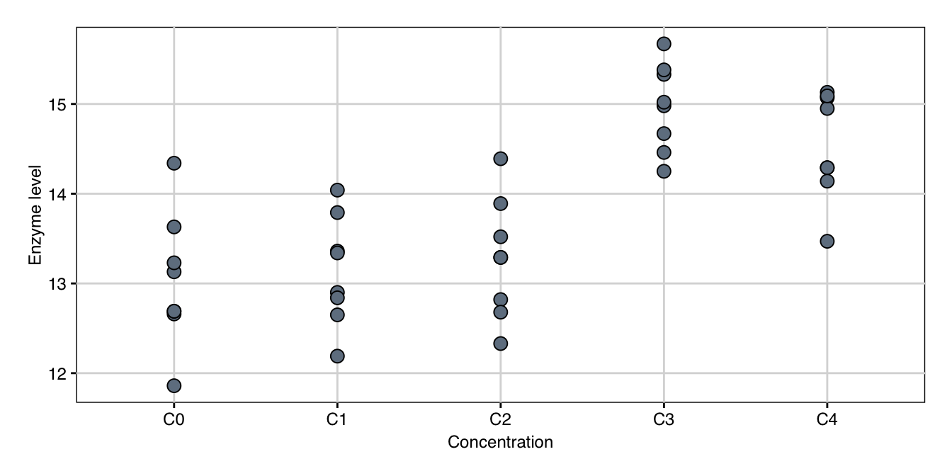
Figure 5.1: Enzyme levels for five increasing concentrations of drug D1.
Trend Analysis using Orthogonal Polynomials
We can analyze such data using ordinary contrasts, but with ordered treatment factor levels, it makes sense to look for trends. We do this using orthogonal polynomials, which are linear, quadratic, cubic, and quartic polynomials that decompose a potential trend into different components. Orthogonal polynomials are formulated as a special set of orthogonal contrasts. We use the emmeans() and contrast() combination again, and ask for a poly contrast to generate the appropriate set of orthogonal contrasts:
m.conc = aov(y~concentration, data=drug_concentrations)
em.conc = emmeans(m.conc, ~concentration)
ct.conc = contrast(em.conc, method="poly")
The contrast weight vectors for our example are shown in Table 5.3.
| Linear | Quadratic | Cubic | Quartic | |
|---|---|---|---|---|
| C0 | -2 | 2 | -1 | 1 |
| C1 | -1 | -1 | 2 | -4 |
| C2 | 0 | -2 | 0 | 6 |
| C3 | 1 | -1 | -2 | -4 |
| C4 | 2 | 2 | 1 | 1 |
Each polynomial contrast measures the similarity of the shape of the data to the pattern described by the weight vector. The linear polynomial measures an upward or downward trend, while the quadratic polynomial measures curvature in the response to the concentrations, such that the trend is not simply a proportional increase or decrease in enzyme level. Cubic and quartic polynomials measure more complex curvature, but become harder to interpret directly.
| Contrast | Estimate | se | df | t value | P(>|t|) |
|---|---|---|---|---|---|
| linear | 4.88 | 0.70 | 35 | 6.95 | 4.38e-08 |
| quadratic | 0.50 | 0.83 | 35 | 0.61 | 5.48e-01 |
| cubic | -2.14 | 0.70 | 35 | -3.05 | 4.40e-03 |
| quartic | -5.20 | 1.86 | 35 | -2.80 | 8.32e-03 |
For our data, we get the result in Table 5.4. We find a highly significant positive linear trend, which means that on average, the enzyme level increases with increasing concentration. The negligible quadratic together with significant cubic and quartic trend components means that there is curvature in the data, but it is changing with the concentration. This reflects the fact that the data show a large increase for the fourth concentration, which then levels off or decreases at the fifth concentration, leading to a sigmoidal pattern.
Time Trends
Another typical example for an ordered factor is time. We have to be careful about the experimental design, however. For example, measuring the enzyme levels at four timepoints using different mice per timepoint can be analyzed using orthogonal polynomials and an analysis of variance approach. This is because each mouse can be randomly allocated to one timepoint, yielding a completely randomized design. If, however, the design is such that the same mice are measured at four different timepoints, then the assumption of random assignment is violated and analysis of variance with contrasts is no longer a reasonable analysis option.4 This type of longitudinal design, where the same unit is followed over time, requires more specialized methods to capture the inherent correlation between timepoints. We briefly discuss simple longitudinal designs in Section 8.4.
Minimal Effective Dose
Another example of contrasts useful for ordered factors are the orthogonal Helmert contrasts. They compare the second level to the first, the third level to the average of the first and second level, the fourth level to the average of the preceding three, and so forth.
Helmert contrasts can be used for finding a minimal effective dose in a dose-response study. Since doses are typically in increasing order, we first test the second-lowest against the lowest dose. If the corresponding average responses cannot be distinguished, we assume that no effect of relevant size is present (provided the experiment is not underpowered). We then pool the data of these two doses and use their common average to compare against the third-smallest dose, thereby increasing the precision compared to contrasting each level only to its preceding level.
Helmert contrasts are not directly available in emmeans, but the package manual tells us how to define them ourselves:
helmert.emmc = function(ordered.levels, ...) {
  # Use built-in R contrast to find contrast matrix
  contrast.matrix = as.data.frame(contr.helmert(ordered.levels))
  # Provide useful name for each contrast
  names(contrast.matrix) = paste(ordered.levels[-1],"vs lower")
  # Provide name of contrast set
  attr(contrast.matrix, "desc") = "Helmert contrasts"
  return(contrast.matrix)
}
In our example data in Figure 5.1, the concentration \(C_3\) shows a clear effect. The situation is much less clear-cut for lower concentrations \(C_0,\dots, C_2\); there might be a hint of linear increase, but this might be due to random fluctuations. Using the Helmert contrasts
ct.helmert = contrast(em.conc, "helmert")yields the contrasts in Table 5.5 and the results in Table 5.6. Concentrations \(C_0, C_1, C_2\) show no discernible differences, while enzyme levels increase significantly for concentration \(C_3\), indicating that the minimal effective dose is between concentrations \(C_2\) and \(C_3\).
| Concentration | C1 vs lower | C2 vs lower | C3 vs lower | C4 vs lower |
|---|---|---|---|---|
| C0 | -1 | -1 | -1 | -1 |
| C1 | 1 | -1 | -1 | -1 |
| C2 | 0 | 2 | -1 | -1 |
| C3 | 0 | 0 | 3 | -1 |
| C4 | 0 | 0 | 0 | 4 |
| Contrast | Estimate | se | df | t value | P(>|t|) |
|---|---|---|---|---|---|
| C1 vs lower | 0.11 | 0.31 | 35 | 0.35 | 7.28e-01 |
| C2 vs lower | 0.38 | 0.54 | 35 | 0.71 | 4.84e-01 |
| C3 vs lower | 5.47 | 0.77 | 35 | 7.11 | 2.77e-08 |
| C4 vs lower | 3.80 | 0.99 | 35 | 3.83 | 5.10e-04 |
5.2.7 Standardized Effect Size
Similar to our previous discussions for simple differences and omnibus \(F\)-tests, we might sometimes profit from a standardized effect size measure for a linear contrast \(\Psi(\mathbf{w})\), which provides the size of the contrast in units of standard deviation.
A first idea is to directly generalize Cohen’s \(d\) as \(\Psi(\mathbf{w})/\sigma_e\) and measure the contrast estimate in units of the standard deviation. A problem with this approach is that the measure still depends on the weight vector: if \(\mathbf{w}=(w_1,\dots,w_k)\) is the weight vector of a contrast, then we can define an equivalent contrast using, for example, \(\mathbf{w}'=2\cdot\mathbf{w}=(2\cdot w_1,\dots,2\cdot w_k)\). Then, \(\Psi(\mathbf{w}')=2\cdot\Psi(\mathbf{w})\), and the above standardized measure also scales accordingly. In addition, we would like our standardized effect measure to equal Cohen’s \(d\) if the contrast describes a simple difference between two groups.
Both problems are resolved by Abelson’s standardized effect size measure \(d_\mathbf{w}\) (Abelson and Prentice 1997): \[ d_\mathbf{w} = \sqrt{\frac{2}{\sum_{i=1}^k w_i^2}}\cdot \frac{\Psi(\mathbf{w})}{\sigma_e} \;\text{estimated by}\; \hat{d}_\mathbf{w}=\sqrt{\frac{2}{\sum_{i=1}^k w_i^2}}\cdot \frac{\hat{\Psi}(\mathbf{w})}{\hat{\sigma}_e}\;. \]
For our scaled contrast \(\mathbf{w}'\), we find \(d_\mathbf{w'}=d_\mathbf{w}\) and the standardized effect sizes for \(\mathbf{w}'\) and \(\mathbf{w}\) coincide. For a simple difference \(\mu_i-\mu_j\), we have \(w_i=+1\) and \(w_j=-1\), all other weights being zero. Thus \(\sum_{i=1}^k w_i^2=2\) and \(d_\mathbf{w}\) is reduced to Cohen’s \(d\).
5.2.8 Power Analysis and Sample Size
The power calculations for linear contrasts can be done based on the contrast estimate and its standard error, which requires calculating the power from the noncentral \(t\)-distribution. We follow the equivalent approach based on the contrast’s sum of squares and the residual variance, which requires calculating the power from the noncentral \(F\)-distribution.
Exact Method
The noncentrality parameter \(\lambda\) of the \(F\)-distribution for a contrast is given as \[ \lambda = \frac{\Psi(\mathbf{w})^2}{\text{Var}(\hat{\Psi}(\mathbf{w}))} = \frac{\left(\sum_{i=1}^k w_i\cdot \mu_i\right)^2}{\frac{\sigma^2}{n}\sum_{i=1}^k w_i^2} = n\cdot 2\cdot \left(\frac{d_\mathbf{w}}{2}\right)^2 = n\cdot 2\cdot f^2_\mathbf{w}\;. \] Note that the last term has exactly the same \(\lambda=n\cdot k\cdot f^2\) form that we encountered previously, since a contrast uses \(k=2\) (sets of) groups and we know that \(f^2=d^2/4\) for direct group comparisons.
From the noncentrality parameter, we can calculate the power for testing the null hypothesis \(H_0: \Psi(\mathbf{w})=0\) for any given significance level \(\alpha\), residual variance \(\sigma_e^2\), sample size \(n\), and assumed real value of the contrast \(\Psi_0\), respectively the assumed standardized effect size \(d_{\mathbf{w},0}\). We calculate the power using our getPowerF() function and increase \(n\) until we reach the desired power.
For our first example contrast \(\mu_1-\mu_2\), we find \(\sum_i w_i^2=2\). For a minimal difference of \(\Psi_0=\) 2 and using a residual variance estimate \(\hat{\sigma}_e^2=\) 1.5, we calculate a noncentrality parameter of \(\lambda=\) 1.33 \(n\). The numerator degree of freedom is df1=1 and the denominator degrees of freedom are df2=n*4-4. For a significance level of \(\alpha=5\%\) and a desired power of \(1-\beta=80\%\), we find a required sample size of \(n=\) 7. We arrive at a very conservative estimate by replacing the residual variance by the upper confidence limit \(\text{UCL}=\) 2.74 of its estimate. This increases the required sample size to \(n=\) 12. The sample size increases substantially to \(n=\) 95 if we want to detect a much smaller contrast value of \(\Psi_0=0.5\).
Similarly, our third example contrast \((\mu_1+\mu_2)/2 - (\mu_3+\mu_4)/2\) has \(\sum_i w_i^2=1\). A minimal value of \(\Psi_0=2\) can be detected with 80% power at a 5% significance level for a sample size of \(n=\) 4 per group, with an exact power of 85% (for \(n=\) 3 the power is 70%). Even though the desired minimal value is identical to the first example contrast, we need less samples since we are comparing the average of two groups to the average of two other groups, making the estimate of the difference more precise.
The overall experiment size is then the maximum sample size required for any contrast of interest.
Portable Power
For making the power analysis for linear contrasts portable, we apply the same ideas as for the omnibus \(F\)-test. The numerator degrees of freedom for a contrast \(F\)-test is \(\text{df}_\text{num}=1\) and we find a sample size formula of \[ n = \frac{2\cdot\phi^2\cdot\sigma_e^2\cdot\sum_{i=1}^k w_i^2}{\Psi_0^2} = \frac{\phi^2}{(d_\mathbf{w}/2)^2} = \frac{\phi^2}{f_\mathbf{w}^2}\;. \] For a simple difference contrast, \(\sum_i w_i^2=2\), we have \(\Psi_0=\delta_0\). With the approximation \(\phi^2\approx 4\) for a power of 80% at a 5% significance level and \(k=2\) factor levels, we derive our old formula again: \(n=16/(\Psi_0/\sigma_e)^2\).
For our first example contrast with \(\Psi_0=2\), we find an approximate sample size of \(n\approx\) 6 based on \(\phi^2=3\), in reasonable agreement with the exact sample size of \(n=\) 7. If we instead ask for a minimal difference of \(\Psi_0=0.5\), this number increases to \(n\approx\) 98 mice per drug treatment group (exact: \(n=\) 95).
The sample size is lower for a contrast between two averages of group means. For our third example contrast with weights \(\mathbf{w}=(1/2, 1/2, -1/2, -1/2)\) we find \(n=8/(\Psi_0/\sigma_e)^2\). With \(\Psi_0=2\), this gives an approximate sample size of \(n\approx\) 5 (exact: 4).
5.3 Multiple Comparisons and Post-Hoc Analyses
5.3.1 Introduction
Planned and Post-Hoc Contrasts
The use of orthogonal contrasts—pre-defined before the experiment is conducted—provides no further difficulty in the analysis. They are, however, often inconvenient for an informative analysis: we may want to use more than \(k-1\) planned contrasts as part of our pre-defined analysis strategy. In addition, exploratory experiments lead to post-hoc contrasts that are based on observed outcomes. Post-hoc contrasts also play a role in carefully planned and executed confirmatory experiments, when peculiar patterns emerge that were not anticipated, but require further investigation.
We must carefully distinguish between planned and post-hoc contrasts: the first case just points to the limitations of independent pre-defined contrasts, but the contrasts and hypotheses are still pre-defined at the planning stage of the experiment and before the data is in. In the second case, we ‘cherry-pick’ interesting results from the data after the experiment is done and we inspected the results. This course of action increases our risk of finding false positives. A common example of a post-hoc contrast occurs when looking at all pair-wise comparisons of treatments and defining the difference between the largest and smallest group mean as a contrast of interest. Since there is always one pair with greatest difference, it is incorrect to use a standard \(t\)-test for this contrast. Rather, the resulting \(p\)-value needs to be adjusted for the fact that we cherry-picked our contrast, making it larger on average than the contrast of any randomly chosen pair. Properly adjusted tests for post-hoc contrasts thus have lower power than those of pre-defined planned contrasts.
The Problem of Multiple Comparisons
Whether we are testing several pre-planned contrasts or post-hoc contrasts of some kind, we also have to adjust our analysis for multiple comparisons.
Imagine a scenario where we are testing \(q\) hypotheses, from \(q\) contrasts, say. We want to control the false positive probability using a significance level of \(\alpha\) for each individual test. The probability that any individual test falsely rejects the null hypothesis of a zero difference is then \(\alpha\). However, even if all \(q\) null hypotheses are true, the probability that at least one of the tests will incorrectly reject its null hypothesis is not \(\alpha\), but rather \(1-(1-\alpha)^q\).
For \(q=200\) contrasts and a significance level of \(\alpha=5\%\), for example, the probability of at least one incorrect rejection is 99.9965%, a near certainty.5 Indeed, the expected number of false positives, given that all 200 null hypotheses are true, is \(200\cdot \alpha=10\). Even if we only test \(q=5\) hypotheses, the probability of at least one incorrect rejection is 22.6% and thus substantially larger than the desired false positive probability.
The probability of at least one false positive in a family of tests (the family-wise or experiment-wise error probability) increases with the number of tests, and in any case exceeds the individual test’s significance level \(\alpha\). This is known as the multiple testing problem. In essence, we have to decide which error we want to control: is it the individual error per hypothesis or is it the overall error of at least one incorrect declaration of significance in the whole family of hypotheses?
A multiple comparison procedure (MCP) is an algorithm that computes adjusted significance levels for each individual test, such that the overall error probability is bound by a pre-defined probability threshold. Some of the procedures are universally applicable, while others a predicated on specific classes of contrasts (such as comparing all pairs), but offer higher power than more general procedures. Specifically, (i) the universal Bonferroni and Bonferroni-Holm corrections provide control for all scenarios of pre-defined hypotheses; (ii) Tukey’s honest significant difference (HSD) provides control for testing all pairs of groups; (iii) Dunnett’s method covers the case of comparing each group to a common control group; and (iv) Scheffé’s method gives confidence intervals and tests for any post-hoc comparisons suggested by the data.
These methods apply generally for multiple hypotheses. Here, we focus on testing \(q\) contrasts \(\Psi(\mathbf{w}_l)\) with \(q\) null hypotheses \[ H_{0,l}: \Psi(\mathbf{w}_l)=0 \] where \(\mathbf{w}_l=(w_{1l},\dots,w_{kl})\) is the weight vector describing the \(l\)th contrast.
5.3.2 General Purpose: Bonferroni-Holm
The Bonferroni and Holm corrections are popular and simple methods for controlling the family-wise error probability. Both work for arbitrary sets of planned contrasts, but are conservative and lead to low significance levels for the individual tests, often much lower than necessary.
The simple Bonferroni method is a single-step procedure to control the family-wise error probability by adjusting the individual significance level from \(\alpha\) to \(\alpha/q\). It does not consider the observed data and rejects the null hypothesis \(H_0: \Psi(\mathbf{w}_l)=0\) if the contrast exceeds the critical value based on the adjusted \(t\)-quantile: \[ \left|\hat{\Psi}(\mathbf{w}_l)\right| > t_{1-\alpha/2q, N-k}\cdot\hat{\sigma}_e\cdot \sqrt{\sum_{i=1}^k\frac{w_{il}^2}{n_i}}\;. \] It is easily applied to existing test results: just multiply the original \(p\)-values by the number of tests \(q\) and declare a test significant if this adjusted \(p\)-value stays below the original significance level \(\alpha\).
For our three example contrasts, we previously found unadjusted \(p\)-values of \(0.019\) for the first, \(0.875\) for the second, and \(10^{-10}\) for the third contrast. The Bonferroni adjustment consists of multiplying each by \(q=3\), resulting in adjusted \(p\)-values of \(0.057\) for the first, \(2.626\) for the second (which we cap at \(1.0\)), and \(3\times 10^{-10}\) for the third contrast, moving the first contrast from significant to not significant at the \(\alpha=5\%\) level. The resulting contrast estimates and \(t\)-test are shown in Table 5.7.
| Contrast | Estimate | se | df | t value | P(>|t|) |
|---|---|---|---|---|---|
| D1-vs-D2 | 1.51 | 0.61 | 28 | 2.49 | 5.66e-02 |
| D3-vs-D4 | -0.10 | 0.61 | 28 | -0.16 | 1.00e+00 |
| Class A-vs-Class B | 4.28 | 0.43 | 28 | 9.96 | 3.13e-10 |
The Bonferroni-Holm method is based on the same assumptions, but uses a multi-step procedure to find an optimal significance level based on the observed data. This increases its power compared to the simple procedure. Let us call the unadjusted \(p\)-values of the \(q\) hypotheses \(p_1,\dots,p_q\). The method first sorts the observed \(p\)-value such that \(p_{(1)}<p_{(2)}<\cdots <p_{(q)}\) and \(p_{(i)}\) is the \(i\)th smallest observed \(p\)-value. It then compares \(p_{(1)}\) to \(\alpha/q\), \(p_{(2)}\) to \(\alpha/(q-1)\), \(p_{(3)}\) to \(\alpha/(q-2)\) and so on until a \(p\)-value exceeds its corresponding threshold. This yields the smallest index \(j\) such that \[ p_{(j)} > \frac{\alpha}{q+1-j}\;, \] and any hypothesis \(H_{0,i}\) for which \(p_i<p_{(j)}\) is declared significant.
5.3.3 Comparisons of All Pairs: Tukey
We gain more power if the set of contrasts has more structure and Tukey’s method is designed for the common case of all pairwise differences. It considers the distribution of the studentized range, the difference between the maximal and minimal group means by calculating honest significant differences (HSD) (Tukey 1949a). It requires a balanced design and rejects \(H_{0,l}: \Psi(\mathbf{w}_l) = 0\) if \[ \left|\hat{\Psi}(\mathbf{w}_l)\right| > q_{1-\alpha,k-1,N}\cdot\hat{\sigma}_e\cdot \sqrt{\frac{1}{2}\sum_{i=1}^k\frac{w_{il}^2}{n}} \quad\text{that is}\quad |\hat{\mu}_i-\hat{\mu}_j| > q_{1-\alpha,k-1,N}\cdot\frac{\hat{\sigma}_e}{\sqrt{n}}\;, \] where \(q_{\alpha,k-1,N}\) is the \(\alpha\)-quantile of the studentized range based on \(k\) groups and \(N=n\cdot k\) samples.
The result is shown in Table 5.8 for our example. Since the difference between the two drug classes is very large, all but the two comparisons within each class yield highly significant estimates, but neither difference of drugs in the same class is significant after Tukey’s adjustment.
5.3.4 Comparisons Against a Reference: Dunnett
Another very common type of biological experiment uses a control group and inference focuses on comparing each treatment with this control group, leading to \(k-1\) contrasts. These contrasts are not orthogonal, and the required adjustment is provided by Dunnett’s method (Dunnett 1955). It rejects the null hypothesis \(H_{0,i}: \mu_i-\mu_1=0\) that treatment group \(i\) shows no difference to the control group 1 if \[ |\hat{\mu}_i-\hat{\mu}_1| > d_{1-\alpha, k-1, N-k}\cdot\hat{\sigma}_e\cdot\sqrt{\frac{1}{n_i}+\frac{1}{n_1}}\;, \] where \(d_{1-\alpha, k-1, N-k}\) is the quantile of the appropriate distribution for this test.
For our example, let us assume that drug \(D1\) is the best current treatment option, and we are interested in comparing the alternatives \(D2\) to \(D4\) to this reference. The required contrasts are the differences from each drug to the reference \(D1\), resulting in Table 5.8.
| Contrast | Estimate | se | df | t value | P(>|t|) |
|---|---|---|---|---|---|
| Pairwise-Tukey | |||||
| D1 - D2 | 1.51 | 0.61 | 28 | 2.49 | 8.30e-02 |
| D1 - D3 | 5.09 | 0.61 | 28 | 8.37 | 2.44e-08 |
| D1 - D4 | 4.99 | 0.61 | 28 | 8.21 | 3.59e-08 |
| D2 - D3 | 3.57 | 0.61 | 28 | 5.88 | 1.45e-05 |
| D2 - D4 | 3.48 | 0.61 | 28 | 5.72 | 2.22e-05 |
| D3 - D4 | -0.10 | 0.61 | 28 | -0.16 | 9.99e-01 |
| Reference-Dunnett | |||||
| D2 - D1 | -1.51 | 0.61 | 28 | -2.49 | 5.05e-02 |
| D3 - D1 | -5.09 | 0.61 | 28 | -8.37 | 1.24e-08 |
| D4 - D1 | -4.99 | 0.61 | 28 | -8.21 | 1.82e-08 |
Unsurprisingly, enzyme levels for drug \(D2\) are barely distinguishable from those of the reference drug \(D1\), and \(D3\) and \(D4\) show very different responses than the reference.
5.3.5 General Purpose and Post-Hoc Contrasts: Scheffé
The method by Scheffé is suitable for testing any group of contrasts, even if they were suggested by the data (Scheffé 1959); in contrast, most other methods are restricted to pre-defined contrasts. Naturally, this freedom of cherry-picking comes at a cost: the Scheffé method is extremely conservative (so effects have to be huge to be deemed significant), and is therefore only used if no other method is applicable.
The Scheffé method rejects the null hypothesis \(H_{0,l}\) if \[ \left|\hat{\Psi}(\mathbf{w}_l)\right| > \sqrt{(k-1) \cdot F_{\alpha,k-1,N-k}} \cdot \hat{\sigma}_e \cdot \sqrt{\sum_{i=1}^k \frac{w_{il}^2}{n_i}}\;. \] This is very similar to the Bonferroni correction, except that the number of contrasts \(q\) is irrelevant, and the quantile is a scaled quantile of an \(F\)-distribution rather than a quantile from a \(t\)-distribution.
For illustration, imagine that our three example contrasts were not planned before the experiment, but rather suggested by the data after the experiment was completed. The adjusted results are shown in Table 5.9.
| Contrast | Estimate | se | df | t value | P(>|t|) |
|---|---|---|---|---|---|
| D1-vs-D2 | 1.51 | 0.61 | 28 | 2.49 | 1.27e-01 |
| D3-vs-D4 | -0.10 | 0.61 | 28 | -0.16 | 9.99e-01 |
| Class A-vs-Class B | 4.28 | 0.43 | 28 | 9.96 | 2.40e-09 |
We notice that the \(p\)-values are much more conservative than with any other method, which reflects the added uncertainty due to the post-hoc nature of the contrasts.
5.3.6 Remarks
There is sometimes disagreement on when multiple comparison corrections are necessary and how strict or conservative they should be. In general, however, results not adjusted for multiple comparisons are unlikely to be accepted without further elaboration. Note that if multiple comparison procedures are required for multiple testing, we also need to adjust quantiles in confidence intervals accordingly.
On the one extreme, it is relatively uncontroversial that sets of post-hoc contrasts always require an appropriate adjustment of the significance levels to achieve reasonable credibility of the analysis. On the other extreme, planned orthogonal contrasts simply partition the treatment factor sum of squares and their hypotheses are independent, so they are usually not adjusted.
Many reasonable sets of contrasts are more nuanced than “every pair” or “everyone against the reference” but still have more structure than an arbitrary set of contrasts. Specialized methods might not exist, while general methods such as Bonferroni-Holm are likely more conservative than strictly required. The analyst’s discretion is then required and the most important aspect is to honestly report what was done, such that others can fully appraise the evidence in the data.
5.4 A Real-Life Example—Drug Metabolization
We further illustrate the one-way ANOVA and use of linear contrasts using a real-life example (Lohasz et al. 2020).6 The two anticancer drugs cyclophosphamide (CP) and ifosfamide (IFF) become active in the human body only after metabolization in the liver by the enzyme CYP3A4, among others. The function of this enzyme is inhibited by the drug ritanovir (RTV), which more strongly affects metabolization of IFF than CP. The experimental setup consisted of 18 independent channels distributed over several microfluidic devices; each channel contained a co-culture of multi-cellular liver spheroids for metabolization and tumor spheroids for measuring drug action.
The experiment used the diameter of the tumor (in \(\mu\text{m}\)) after 12 days as the response variable. There are six treatment groups: a control condition without drugs, a second condition with RTV alone, and the four conditions CP only, IFF only, and the combined CP:RTV and IFF:RTV. The resulting data are shown in Figure 5.2A for each channel.
A preliminary analysis revealed that device-to-device variation and variation from channel to channel were negligible compared to the within-channel variance, and these two factors were consequently ignored in the analysis. Thus, data are pooled over the channels for each treatment group and the experiment is analyzed as a (slightly unbalanced) one-way ANOVA. We discuss an alternative two-way ANOVA in Section 6.3.8.
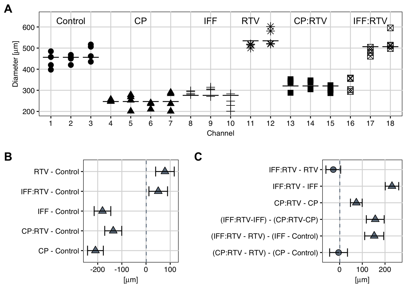
Figure 5.2: A: Observed diameters by channel. Point shape indicates treatment. Channel 16 appears to be mislabelled. B: Estimated treatment-versus-control contrasts and Dunnett-adjusted 95%-confidence intervals based on data excluding channel 16, significant contrasts are indicated as triangles. C: As (B) for specific (unadjusted) contrasts of interest.
Inhomogeneous Variances
The omnibus \(F\)-test and linear contrast analysis require equal within-group variances between treatment groups. This hypothesis was tested using the Levene test and a \(p\)-value below 0.5% indicated that variances might differ substantially. If true, this would complicate the analysis. Looking at the raw data in Figure 5.2A, however, reveals a potential error in channel 16, which was labelled as IFF:RTV, but shows tumor diameters in excellent agreement with the neighboring CP:RTV treatment. Including channel 16 in the IFF:RTV group then inflates the variance estimate. It was therefore decided to remove channel 16 from further analysis, the hypothesis of equal variances is then no longer rejected (\(p>0.9\)), and visual inspection of the data confirms that dispersions are very similar between channels and groups.
Analysis of Variance
As is expected from looking at the data in Figure 5.2A, the one-way analysis of variance of tumor diameter versus treatment results in a highly significant treatment effect.
| Df | Sum Sq | Mean Sq | F value | Pr(>F) | |
|---|---|---|---|---|---|
| Condition | 5 | 815204.9 | 163040.98 | 154.53 | 6.34e-33 |
| Residuals | 60 | 63303.4 | 1055.06 |
The effect sizes are an explained variation of \(\eta^2=\) 93%, a standardized effect size of \(f^2=\) 12.88, and a raw effect size of \(b^2=\) 13589.1\(\mu\text{m}^2\) (an average deviation between group means and general mean of \(b=\) 116.57\(\mu\text{m}\))
Linear Contrasts
Since the \(F\)-test does not elucidate which groups differ and by how much, we proceed with a more targeted analysis using linear contrasts to estimate and test meaningful and interpretable comparisons. With a first set of standard contrasts, we compare each treatment group to the control condition. The resulting contrast estimates are shown in Figure 5.2B together with their Dunnett-corrected 95%-confidence intervals.
Somewhat surprisingly, the RTV-only condition shows tumor diameters significantly larger than those under the control condition, indicating that RTV alone influences the tumor growth. Both conditions involving CP show reduced tumor diameters, indicating that CP inhibits tumor growth, as does IFF alone. Lastly, RTV seems to substantially decrease the efficacy of IFF, leading again to tumor diameters larger than under the control condition, but (at least visually) comparable to the RTV condition.
The large and significant difference between control and RTV-only poses a problem for the interpretation: we are interested in comparing CP:RTV against CP-only and similarly for IFF. But CP:RTV could be a combined effect of tumor diameter reduction by CP (compared to control) and increase by RTV (compared to control). We have two options for defining a meaningful contrast: (i) estimate the difference in tumor diameter between CP:RTV and CP. This is a comparison between the combined and single drug actions. Or (ii) estimate the difference between the change in tumor diameter from CP to control and the change from CP:RTV to RTV (rather than to control). This is a comparison between the baseline tumor diameters under control and RTV to those under addition of CP and is the net-effect of CP (provided that RTV increases tumor diameters equally with and without CP).
The two sets of comparisons lead to different contrasts, but both are meaningful for these data. The authors of the study decided to go for the first type of comparison and compared tumor diameters for each drug with and without inhibitor. The two contrasts are \(\text{IFF:RTV}-\text{IFF}\) and \(\text{CP:RTV}-\text{CP}\), shown in rows 2 and 3 of Figure 5.2C. Both contrasts show a large and significant increase in tumor diameter in the presence of the inhibitor RTV, where the larger loss of efficacy for IFF yields a more pronounced difference.
For a complete interpretation, we are also interested in comparing the two differences between the CP and the IFF conditions: is the reduction in tumor diameter under CP smaller or larger than under IFF? This question addresses a difference of differences, a very common type of comparison in biology, when different conditions are contrasted and a ‘baseline’ or control is available for each condition. We express this question as \((\text{IFF:RTV}-\text{IFF}) - (\text{CP:RTV}-\text{CP})\), and we can sort the terms to derive the contrast form \((\text{IFF:RTV}+\text{CP}) - (\text{CP:RTV}+\text{IFF})\). Thus, we use weights of \(+1\) for the treatment groups IFF:RTV and CP, and weights of \(-1\) for the groups CP:RTV and IFF to define the contrast. Note that this differs from our previous example contrast comparing drug classes, where we compared averages of several groups by using weights \(\pm 1/2\). The estimated contrast and confidence interval is shown in the fourth row in Figure 5.2C: the two increases in tumor diameter under co-administered RTV are significantly different, with about 150 \(\mu\text{m}\) more under IFF than under CP.
For comparison, the remaining two rows in Figure 5.2C show the tumor diameter increase for each drug with and without inhibitor, where the no-inhibitor condition is compared to the control condition, but the inhibitor condition is compared to the RTV-only condition. Now, IFF shows less increase in tumor diameter than in the previous comparison, but the result is still large and significant. In contrast, we do not find a difference between the CP and CP:RTV conditions indicating that loss of efficacy for CP is only marginal under RTV. This is because the previously observed difference can be explained by the difference in ‘baseline’ between control and RTV-only. The contrasts are constructed as before: for CP, the comparison is \((\text{CP:RTV}-\text{RTV}) - (\text{CP}-\text{Control})\) which is equivalent to \((\text{CP:RTV}+\text{Control}) - (\text{RTV} + \text{CP})\).
Conclusion
What started as a seemingly straightforward one-way ANOVA turned into a much more intricate analysis. Only the direct inspection of the raw data revealed the source of the heterogeneous treatment group variances. The untestable assumption of a mislabelling followed by removal of the data from channel 16 still led to a straightforward omnibus \(F\)-test and ANOVA table.
Great care is also required in the more detailed contrast analysis. While the RTV-only condition was initially thought to provide another control condition, a comparison with the empty control revealed a systematic and substantial difference, with RTV-only showing larger tumor diameters. Two sets of contrasts are then plausible, using different ‘baseline’ values for estimating the effect of RTV in conjunction with a drug. Both sets of contrasts have straightforward interpretations, but which set is more meaningful depends on the biological question. Note that the important contrast of tumor diameter differences between inhibited and uninhibited conditions compared between the two drugs is independent of this decision.
5.5 Notes and Summary
Notes
Linear contrasts for finding minimum effective doses are discussed in Ruberg (1989), and general design and analysis of dose finding studies in Ruberg (1995a) and Ruberg (1995b).
If and when multiple comparison procedures are required is sometimes a matter of debate. Some people argue that such adjustments are rarely called for in designed experiments (Finney 1988; O’Brien 1983). Further discussion of this topic is provided in Cox (1965), O’Brien (1983), Curran-Everett (2000), and Noble (2009). An authoritative treatment of the issue is Tukey (1991). A book-length treatment is Rupert Jr (2012).
In addition to the weak and strong control family-wise error (Proschan and Brittain 2020), we can also control for other types of error (Lawrence 2019), most prominently the false discovery rate FDR (Benjamini and Hochberg 1995). A relatively recent graphical method allows adapting the Bonferroni-Holm procedure to a specific set of hypotheses and can yield less conservative adjustments (Bretz et al. 2009).
Using R
Estimation of contrasts in R is discussed in Section 5.2.4. A very convenient option for applying multiple comparisons procedures is to use the emmeans package and follow the same strategy as before: estimate the model parameters using aov() and estimate the group means using emmeans(). We can then use the contrast() function with an adjust= argument to choose a multiple correction procedure to adjust \(p\)-values and confidence intervals of contrasts. This function also has several frequently used sets of contrasts built-in, such as method="pairwise" for generating all pairwise contrasts or method="trt.vs.ctrl1" and method="trt.vs.ctrlk" for generating contrasts comparing all treatments to the first, respectively last, level of the treatment factor. For estimated marginal means em, and either the corresponding built-in contrasts or our manually defined set of contrasts ourContrasts, we access the five procedures as
contrast(em, method=ourContrasts, adjust="bonferroni")
contrast(em, method=ourContrasts, adjust="holm")
contrast(em, method="pairwise", adjust="tukey")
contrast(em, method="trt.vs.ctrl1", adjust="dunnett")
contrast(em, method=ourContrasts, adjust="scheffe")
By default, these functions provide the contrast estimates and associated \(t\)-tests. We can use the results of contrast() as an input to confint() to get contrast estimates and their adjusted confidence intervals instead.
The package Superpower provides functionality to perform power analysis of contrasts in conjunction with emmeans.
Summary
Linear contrasts are a principled way for defining comparisons between two sets of group means and constructing the corresponding estimators, their confidence intervals, and \(t\)-statistics. While an ANOVA omnibus \(F\)-test looks for any pattern of deviation between group means, linear contrasts use specific comparisons and are more powerful in detecting the specified deviations. Without much exaggeration, linear contrasts are the main reason for conducting comparative experiments and their definition is an important part of an experimental design.
With more than one hypothesis tested, multiple comparison procedures are often required to adjust for the inflation in false positives. General purpose procedures are easy to use, but sets of contrasts often have more structure that can be exploited to gain more power.
Power analysis for contrasts poses no new problems, but the adjustments by MCPs can only be considered for single-step procedures, because multi-step procedures depend on the observed \(p\)-values which are of course unknown at the time of planning the experiment.
We can do this using a ‘contrast’ \(\mathbf{w}=(1/k,1/k,\dots,1/k)\), even though its weights do not sum to zero.↩︎
A small subtlety arises from estimating the contrasts: since all \(t\)-tests are based on the same estimate of the residual variance, the tests are still statistically dependent. The effect is usually so small that we ignore this subtlety in practice.↩︎
It is plausible that measurements on the same mouse are more similar between timepoints close together than between timepoints further apart, a fact that ANOVA cannot properly capture.↩︎
If 200 hypotheses seems excessive, consider a simple microarray experiment: here, the difference in expression level is simultaneously tested for thousands of genes.↩︎
The authors of this study kindly granted permission to use their data. Purely for illustration, we provide some alternative analyses to those in the publication.↩︎