Chapter 2 Review of Statistical Concepts

2.1 Introduction

We briefly review some basic concepts in statistical inference for analyzing a given set of data. The material roughly covers a typical introductory course in statistics: describing variation, estimating parameters, and testing hypotheses in the context of normally distributed data. The focus on the normal distribution avoids the need for more advanced mathematical and computational machinery and allows us to concentrate on the design rather than complex analysis aspects of an experiment in later chapters.

2.2 Probability

2.2.1 Random Variables and Distributions

Even under well controlled conditions, replicate measurements will deviate from each other to a certain degree. In biological experiments, for example, two main sources of this variation are heterogeneity of the experimental material and measurement uncertainties. After accounting for potential systematic effects, we can assign probabilities to these deviations.

A random variable maps a random event to a number, for example to a (random) deviation of an observed measurement from the underlying true value. One often denotes a random variable by a capital letter and a specific realization or outcome by the corresponding lower case letter. For example, we might be interested in the level of a specific liver enzyme in mouse serum. The data in Table 2.1 show again the measured levels of ten randomly selected mice, where one sample was taken from each mouse, processed using the kit from vendor A, and the enzyme level was quantified using a well-established assay.

Table 2.1: Measured enzyme levels of ten randomly selected mice.

1	2	3	4	5	6	7	8	9	10
8.96	8.95	11.37	12.63	11.38	8.36	6.87	12.35	10.32	11.99

We formally describe the observation for the \(i\)th mouse by the outcome \(y_i\) of its associated random variable \(Y_i\). The (probability) distribution of a random variable \(Y\) gives the probability of observing an outcome within a given interval. The probability density function (pdf) \(f_Y(y)\) and the cumulative distribution function (cdf) \(F_Y(y)\) of \(Y\) both describe its distribution. The area under the pdf between two values \(a\) and \(b\) gives the probability that a realization of \(Y\) falls into the interval \([a,\,b]\): \[ \mathbb{P}(Y\in [a,\,b]) = \mathbb{P}(a\leq Y\leq b) = \int_a^b f_Y(y')\,dy' = F_Y(b)-F_Y(a)\;, \] while the cdf gives the probability that \(Y\) will take any value lower or equal to \(y\): \[ F_Y(y) = \mathbb{P}(Y \leq y) = \int_{-\infty}^y f_Y(y') dy'\;. \] It is often reasonable to assume a normal (or Gaussian) distribution for the data. This distribution has two parameters \(\mu\) and \(\sigma^2\) and its probability density function is \[ f_Y(y;\mu,\sigma^2) = \frac{1}{\sqrt{2\pi}\sigma}\cdot\exp\left(-\frac{1}{2}\cdot\left(\frac{y-\mu}{\sigma}\right)^2\right)\;, \] which yields the famous bell-shaped curve symmetric around a peak at \(\mu\) and with width determined by \(\sigma\). In our example, we have normally distributed observations with \(\mu=10\) and \(\sigma^2=2\), which corresponds to the probability density function shown in Figure 2.1.

We write \(Y\sim N(\mu,\sigma^2)\) to say that the random variable \(Y\) has a normal distribution with parameters \(\mu\) and \(\sigma^2\). The density is symmetric around \(\mu\) and thus the probability that we observe an enzyme level lower than 10 is \(\mathbb{P}(Y\leq 10)=0.5\) in our example. The probability that the observed level falls above \(a=\) 12.7 is about \(1-F_Y(a)=\int_{a}^\infty f_Y(y')dy'=0.025\) or 2.5%. More details on normal distributions and their properties are given in Section 2.2.6.

2.2.2 Quantiles

We are often interested in the \(\alpha\)-quantile \(q_\alpha\) below which a realization falls with given probability \(\alpha\) such that \[ \mathbb{P}(Y\leq q_\alpha)=\alpha\;. \] The value \(q_\alpha\) depends on the distribution of \(Y\) and different distributions have different quantiles for the same \(\alpha\).

For our example, a new observation will be below the quantile \(q_{0.025}=\) 7.3 with probability \(2.5\%\) and below \(q_{0.975}=\) 12.7 with probability \(97.5\%\). These two quantiles are indicated by arrows in Figure 2.1 and each shaded area corresponds to a probability of \(2.5\%\).

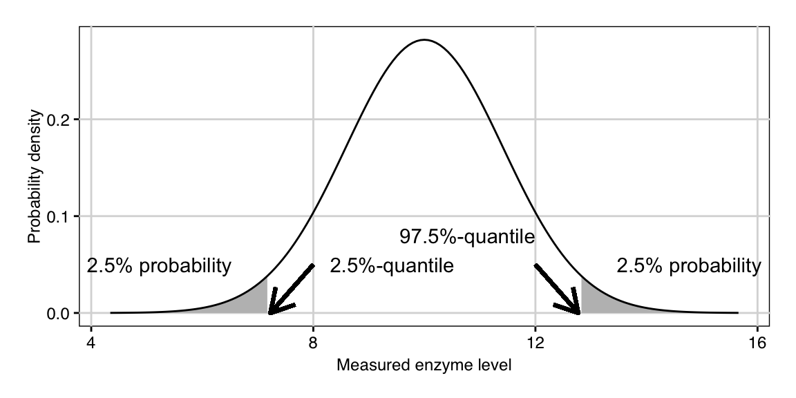
Figure 2.1: Normal density for \(N(\mu=10,\,\sigma^2=2)\) with 2.5% and 97.5-%-quantiles (arrows) and areas corresponding to 2.5-% probability under left and right tail (grey shaded areas).

2.2.3 Independence and Conditional Distributions

The joint distribution of two random variables \(X\) and \(Y\) is denoted \[ F_{X,Y}(x,y)=\mathbb{P}(X\leq x, Y\leq y) = \mathbb{P}(X\leq x)\cdot\mathbb{P}(Y\leq y | X\leq x)\;, \] and is the probability that \(X\leq x\) and \(Y\leq y\) are simultaneously true. We can decompose it into the marginal distribution \(\mathbb{P}(X\leq x)\) and the conditional distribution \(\mathbb{P}(Y\leq y | X\leq x)\). The conditional distribution is read as “\(Y\) given \(X\)” and gives the probability that \(Y\leq y\) if we know that \(X\leq x\).

In our example, the enzyme levels \(Y_i\) and \(Y_j\) of two different mice are independent: their realizations \(y_i\) and \(y_j\) are both from the same distribution, but knowing the measured level of one mouse will tell us nothing about the level of the other mouse, hence \(\mathbb{P}(Y_i\leq y_i \,|\, Y_j\leq y_j)=\mathbb{P}(Y_i\leq y_i)\).

The joint probability of two independent variables is the product of the two individual probabilities. For example, the probability that both mouse \(i\) and mouse \(j\) yield measurements below 10 is \(\mathbb{P}(Y_i\leq 10,\, Y_j\leq 10)=\mathbb{P}(Y_i\leq 10\,|\, Y_j\leq 10)\cdot\mathbb{P}(Y_j\leq 10)=\mathbb{P}(Y_i\leq 10)\cdot\mathbb{P}(Y_j\leq 10)=0.5\cdot 0.5=0.25\).

As an example of two dependent random variables, we might take a second sample from each mouse and measure the enzyme level of this sample, similar to Figure 1.1B. The resulting data are shown in Table 2.2. We immediately observe that the first and second measurements from the same mouse are much more similar than any measurements from two different mice.

Table 2.2: Measured enzyme levels of 10 lab mice, each mouse measured twice.

1	2	3	4	5	6	7	8	9	10
8.96	8.95	11.37	12.63	11.38	8.36	6.87	12.35	10.32	11.99
8.82	9.13	11.37	12.50	11.75	8.65	7.63	12.72	10.51	11.80

We denote by \(Y_{i,1}\) and \(Y_{i,2}\) the two measurements of the \(i\)th mouse. Then, \(Y_{i,1}\) and \(Y_{j,1}\) are independent since they are measurements of two different mice and \(\mathbb{P}(Y_{i,1}\leq 10|Y_{j,1}\leq 10)=\mathbb{P}(Y_{i,1}\leq 10)=0.5\), for example. In contrast, \(Y_{i,1}\) and \(Y_{i,2}\) are not independent, because they are two measurements of the same mouse: knowing the result of the first measurement gives us a strong indication about the value of the second measurement and \(\mathbb{P}(Y_{i,2}\leq 10|Y_{i,1}\leq 10)\) is likely to be much higher than 0.5, because if the first sample yields a level below 10, the second will also tend to be below 10. We discuss this in more detail shortly when we look at covariances and correlations.

2.2.4 Expectation and Variance

Instead of working with the full distribution of a random variable \(Y\), it is often sufficient to summarize its properties by the expectation and variance, which roughly speaking give the position around which the density function spreads, and the dispersion of values around this position, respectively.

The expected value (or expectation, also called mean or average) of a random variable \(Y\) is a measure of its location. It is defined as the weighted average of all possible realizations \(y\) of \(Y\), which we calculate by integrating over the values \(y\) and multiplying each value with the probability density \(f_Y(y)\) of \(Y\)’s distribution: \[ \mathbb{E}(Y) = \int_{-\infty}^{+\infty} y\cdot f_Y(y)\, dy\;. \]

The expectation is linear and the following arithmetic rules apply for any two random variables \(X\) and \(Y\) and any non-random constant \(a\): \[\begin{equation*} \mathbb{E}(a) = a \,,\; \mathbb{E}(a+X) = a+\mathbb{E}(X) \,,\; \mathbb{E}(a\cdot X) = a\cdot\mathbb{E}(X)\,,\; \mathbb{E}(X+Y) = \mathbb{E}(X)+\mathbb{E}(Y). \end{equation*}\] If \(X\) and \(Y\) are independent, then the expectation of their product is the product of the expectations: \[\begin{equation*} \mathbb{E}(X\cdot Y) = \mathbb{E}(X)\cdot \mathbb{E}(Y)\;, \end{equation*}\] but note that in general \(\mathbb{E}\left(X \,/\, Y\right) \not= \mathbb{E}(X) \,/\, \mathbb{E}(Y)\) even for independent variables. The expectation is often denoted by \(\mu\).

The variance of a random variable \(Y\), often denoted by \(\sigma^2\), is defined as \[ \text{Var}(Y) = \mathbb{E}\left(\left(Y-\mathbb{E}(Y)\right)^2\right)=\mathbb{E}(Y^2)-\mathbb{E}(Y)^2\;, \] the expected distance of a value of \(Y\) from its expectation, where the distance is measured as the squared difference. It is a measure of dispersion, describing how wide values spread around their expected value.

For a non-random constant \(a\) and two random variables \(X\) and \(Y\), the following arithmetic rules apply for variances: \[\begin{equation*} \text{Var}(a) = 0\,,\;\text{Var}(a + Y) = \text{Var}(Y)\,,\;\text{Var}(a\cdot Y) = a^2\cdot\text{Var}(Y)\;. \end{equation*}\] If \(X\) and \(Y\) are independent, then \[\begin{equation*} \text{Var}(X+Y) = \text{Var}(X)+\text{Var}(Y)\;. \end{equation*}\] Moreover, the variance of the difference of two independent random variables is larger than each individual variance since \[\begin{equation*} \text{Var}(X-Y) = \text{Var}(X+(-1)\cdot Y) = \text{Var}(X)+(-1)^2\cdot\text{Var}(Y) = \text{Var}(X)+\text{Var}(Y). \end{equation*}\]

For a normally distributed random variable \(Y\sim N(\mu,\sigma^2)\), the expectation and variance completely specify the full distribution, since \(\mu=\mathbb{E}(Y)\) and \(\sigma^2=\text{Var}(Y)\). For our example distribution in Figure 2.1, the expectation \(\mu=10\) provides the location of the maximum of the density, and the variance \(\sigma^2=2\) corresponds to the width of the density curve around this location. The relation between a distribution’s parameters and its expectation and variance is less direct for many other distributions.

Given the expectation and variance of a random variable \(Y\), we can define a new random variable \(Z\) with expectation zero and variance one by shifting and scaling: \[ Z=\frac{Y-\mathbb{E}(Y)}{\sqrt{\text{Var}(Y)}}\quad\text{ has }\quad \mathbb{E} (Z)=0 \text{ and } \text{Var}(Z)=1\;. \] If \(Y\) is normally distributed with parameters \(\mu\) and \(\sigma^2\), then \(Z=(Y-\mu)/\sigma\) is also normally distributed with parameters \(\mu=0\) and \(\sigma^2=1\). In general, however, the distribution of \(Z\) will be of a different kind than the distribution of \(Y\). For example, \(Y\) might be a concentration and take only positive values, but \(Z\) is centered around zero and will take positive and negative values.

The realizations of \(n\) independent and identically distributed random variables \(Y_i\) are often summarized by their arithmetic mean \(\bar{Y}=\frac{1}{n}\sum_{i=1}^n Y_i\). Since \(\bar{Y}\) is a function of random variables, it is itself a random variable and therefore has a distribution. Indeed, if the individual \(Y_i\) are normally distributed, then \(\bar{Y}\) also has a normal distribution. Assuming that all \(Y_i\) have expectation \(\mu\) and variance \(\sigma^2\), we can determine the expectation and variance of the arithmetic mean. First, we find that its expectation is identical to the expectation of the individual \(Y_i\): \[ \mathbb{E}(\bar{Y}) = \mathbb{E}\left(\frac{1}{n}\sum_{i=1}^n Y_i\right) = \frac{1}{n}\sum_{i=1}^n \mathbb{E}(Y_i) = \frac{1}{n}\sum_{i=1}^n \mu = \frac{1}{n}\cdot n\cdot\mu=\mu\;. \] However, its variance is smaller than the individual variances, and decreases with the number of random variables: \[ \text{Var}(\bar{Y}) = \text{Var}\left(\frac{1}{n}\sum_{i=1}^n Y_i\right) = \frac{1}{n^2}\sum_{i=1}^n\text{Var}(Y_i) = \frac{1}{n^2}\cdot n\cdot \sigma^2 = \frac{\sigma^2}{n}\;. \] For our example, the average of the ten measurements of enzyme levels has expectation \(\mathbb{E}(\bar{Y})=\mathbb{E}(Y_i)=10\), but the variance \(\text{Var}(\bar{Y})=\sigma^2/10=\) 0.2 is only one-tenth of the individual variances \(\text{Var}(Y_i)=\sigma^2=\) 2. The average of ten measurements therefore shows less dispersion around the mean than each individual measurement. Since the sum of normally distributed random variables is again normally distributed, we thus know that \(\bar{Y}\sim N(\mu, \sigma^2/n)\) with \(n=10\) for our example.

We often describe the scale of the distribution by the standard deviation: \[ \text{sd}(Y)=\sqrt{\text{Var}(Y)}\;, \] which is a measure of dispersion in the same unit as the random variable. While the variance of the sum of independent random variables is the sum of their variances, the variance does not behave nicely with changes in the measurement scale: if \(Y\) is measured in meters, its variance is given in square-meters. A shift to centimeters then multiplies all measurements by 100, but the variance by \(100^2=10\,000\). In contrast, the standard deviation behaves nicely under changes in scale, but not under addition: \[\begin{equation*} \text{sd}(a\cdot Y) = |a|\cdot\text{sd}(Y) \quad\text{but}\quad \text{sd}(X\pm Y) = \sqrt{\text{sd}(X)^2+\text{sd}(Y)^2}\;, \end{equation*}\] for independent \(X\) and \(Y\). For our example, \(\text{sd}(Y_i)=\) 1.41 and \(\text{sd}(\bar{Y})=\) 0.45.

2.2.5 Covariance and Correlation

The joint dispersion of \(X\) and \(Y\) is described by their covariance \[ \text{Cov}(X,Y) = \mathbb{E}\Big((X-\mathbb{E}(X))\cdot(Y-\mathbb{E}(Y))\Big) = \mathbb{E}(X\cdot Y)-\mathbb{E}(X)\cdot\mathbb{E}(Y)\;, \] which measures the dependency between \(X\) and \(Y\): the covariance is large and positive if a large deviation of \(X\) from its expectation is associated with a large deviation of \(Y\) in the same direction; it is large and negative if these directions are reverse.

The covariance of a random variable with itself is its variance \(\text{Cov}(X,X)=\text{Var}(X)\) and the covariance is zero if \(X\) and \(Y\) are independent (the converse is not true!). The covariance is linear in both arguments, in particular: \[\begin{equation*} \text{Cov}(a\cdot X+b\cdot Y,\, Z) = a\cdot\text{Cov}(X,\,Z)+b\cdot\text{Cov}(Y,\,Z)\;, \end{equation*}\] and similarly for the second argument. A related measure is the correlation \[ \text{Corr}(X,Y) = \frac{\text{Cov}(X,Y)}{\text{sd}(X)\cdot\text{sd}(Y)}\;, \] which is a unit-less number between \(-1\) and \(+1\).

The covariance is the missing ingredient to extend our formulas for the expectation and variance to the case of two dependent variables by \[ \mathbb{E}(X\cdot Y) = \mathbb{E}(X)\cdot\mathbb{E}(Y)+\text{Cov}(X,Y) \] and \[\begin{align*} \text{Var}(X+Y) &= \text{Var}(X) + \text{Var}(Y) + 2\cdot \text{Cov}(X,Y) \\ \text{Var}(X-Y) &= \text{Var}(X) + \text{Var}(Y) - 2\cdot \text{Cov}(X,Y)\;, \end{align*}\] which both reduce to the previous formulas if the variables are independent and \(\text{Cov}(X,Y)=0\).

In our first example, the measurements of enzyme levels in ten mice are independent. Therefore, \(\text{Cov}(Y_i,Y_i)=\text{Var}(Y_i)\) and \(\text{Cov}(Y_i,Y_j)=0\) for two different mice \(i\) and \(j\).

In our second example, two samples were measured for each mouse. We can write the random variable \(Y_{i,j}\) for the \(j\)th measurement of the \(i\)th mouse as the sum of a random variable \(M_i\) capturing the difference of the true enzyme level of mouse \(i\) to the expectation \(\mu=10\), and a random variable \(S_{i,j}\) capturing the difference between the observed enzyme level \(Y_{i,j}\) and the true level of mouse \(i\). Then, \[ Y_{i,j} = \mu + M_i + S_{i,j}\;, \] where \(\mu=10\), \(M_i\sim N(0,\sigma_m^2)\) and \(S_{i,j}\sim N(0,\sigma_e^2)\). The \(i\)th mouse then has average response \(\mu+M_i\), and the first measurement deviates from this by \(S_{i,1}\). If \(M_i\) and \(S_{i,j}\) are all independent, then the overall variance \(\sigma^2\) is decomposed into the two variance components: \(\text{Var}(Y_{i,j})=\sigma^2=\sigma_m^2+\sigma_e^2=\text{Var}(M_i)+\text{Var}(S_{i,j})\).

If we plot the two measurements \(Y_{i,1}\) and \(Y_{i,2}\) of each mouse in a scatter-plot as in Figure 2.2A, we notice the high correlation: whenever the first measurement is high, the second measurement is also high. The covariance between these variables is \[\begin{align*} & \text{Cov}(Y_{i,1}\,,Y_{i,2}) \\ &= \text{Cov}(\mu+M_i+S_{i,1}\,,\mu+M_i+S_{i,2}) \\ &= \text{Cov}(M_i+S_{i,1}\,,M_i+S_{i,2}) \\ & = \underbrace{\text{Cov}(M_i\,,M_i)}_{=\text{Var}(M_i)} + \underbrace{\text{Cov}(M_{i}\,,S_{i,2})}_{=0\text{ (independence)}} + \underbrace{\text{Cov}(S_{i,1}\,,M_{i})}_{=0\text{ (independence)}} + \underbrace{\text{Cov}(S_{i,1}\,,S_{i,2})}_{=0\text{ (independence)}} \\ & = \sigma_m^2\;, \end{align*}\] and the correlation is \[\begin{equation*} \text{Corr}(Y_{i,1},Y_{i,2}) = \frac{\text{Cov}(Y_{i,1},Y_{i,2})}{\text{sd}(Y_{i,1})\cdot\text{sd}(Y_{i,2})} = \frac{\sigma_m^2}{\sigma_m^2+\sigma_e^2}\;. \end{equation*}\] With \(\sigma_m^2=\) 1.9 and \(\sigma_e^2=\) 0.1, the correlation is extremely high at 0.95. This can also be seen in Figure 2.2B, which shows the two measurements for each mouse separately. Here, the magnitude of the differences between the individual mice (grey points) is measured by \(\sigma_m^2\), while the magnitude of differences between the two measurements of any mouse (plus and cross) is much smaller and is given by \(\sigma_e^2\).

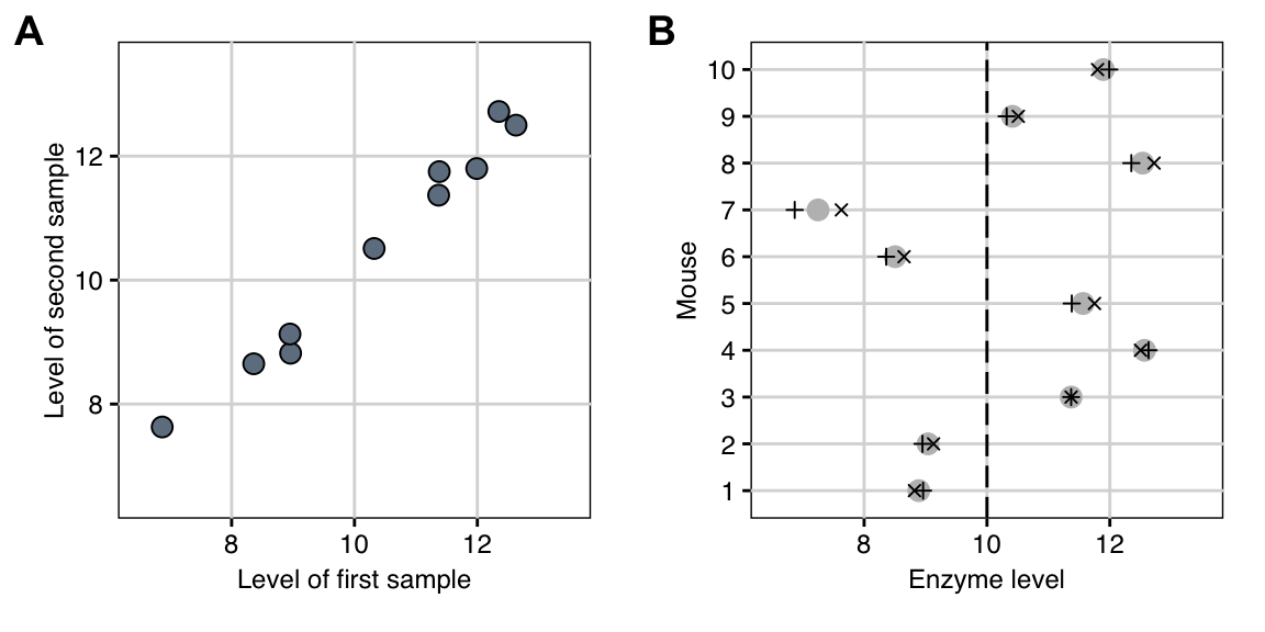
Figure 2.2: A: Scatterplot of the enzyme levels of the first and second sample for each mouse. The points lie close to a line, indicating a very high correlation between the two samples. B: Average (grey) and first (plus) and second (cross) sample enzyme level for each mouse. The dashed line is the average level in the mouse population.

As a third example, we consider the arithmetic mean of independent random variables and determine the covariance \(\text{Cov}(Y_i,\bar{Y})\). Because \(\bar{Y}\) is computed using \(Y_i\), these two random variables cannot be independent and we expect a non-zero covariance. Using the linearity of the covariance, we get: \[\begin{equation*} \text{Cov}(Y_i,\bar{Y}) = \text{Cov}\left(Y_i,\frac{1}{n}\sum_{j=1}^n Y_j\right) = \frac{1}{n}\sum_{j=1}^n \text{Cov}(Y_i,Y_j) = \frac{1}{n} \text{Cov}(Y_i,Y_i) = \frac{\sigma^2}{n}\;, \end{equation*}\] using the fact that \(\text{Cov}(Y_i,Y_j)=0\) for \(i\not=j\). Thus, the covariance decreases with increasing number of random variables, because the variation of the average \(\bar{Y}\) depends less and less on each single variable \(Y_i\).

2.2.6 Some Important Distributions

We encounter four families of distributions in the next chapters, and briefly gather some of their properties here for future reference. We assume that all data follow some normal distribution describing the errors due to sampling and measurement, for example. Derived from that are (i) the \(\chi^2\)-distribution related to estimates of variance, (ii) the \(F\)-distribution related to the ratio of two variance estimates, and (iii) the \(t\)-distribution related to estimates of means and differences in means.

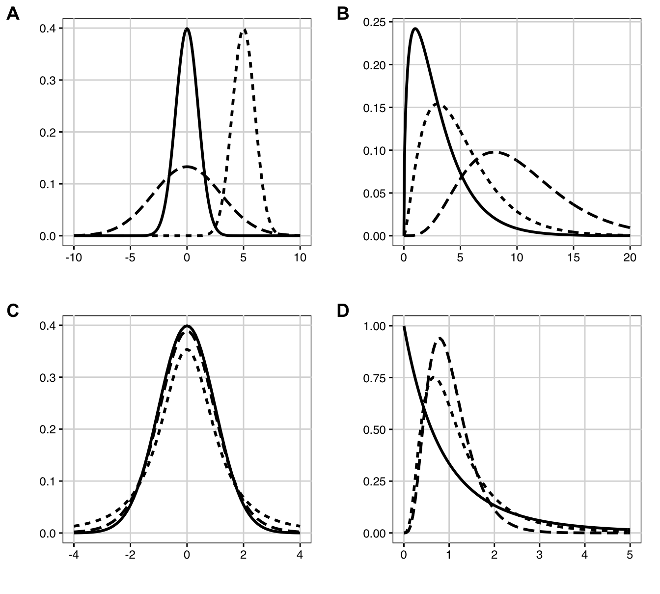
Figure 2.3: Probability densities. A: Normal distributions: standard normal with mean \(\mu=0\), standard deviation \(\sigma=1\) (solid); shifted: \(\mu=5\), \(\sigma=1\) (dotted); scaled: \(\mu=0\), \(\sigma=3\) (dashed). B: \(\chi^2\)-distributions with 3 (solid), 5 (dotted) and 10 (dashed) degrees of freedom. C: \(t\)-distributions with 2 (dotted) and 10 (dashed) degrees of freedom and standard normal density (solid). D: \(F\)-distributions with \((n=2, m=10)\) numerator/denominator degrees of freedom (solid), respectively \((n=10, m=10)\) (dotted) and \((n=10, m=100)\) (dashed).

Normal Distribution

The normal distribution is well-known for its bell-shaped density, shown in Figure 2.3A for three combinations of its two parameters \(\mu\) and \(\sigma^2\). The special case of \(\mu=0\) and \(\sigma^2=1\) is called the standard normal distribution.

The omnipresence of the normal distribution can be partly explained by the central limit theorem, which states that if we have a sequence of random variables with identical distribution (for example, describing the outcome of many measurements), then their average will have a normal distribution, no matter what distribution each single random variable has. Technically, if \(Y_1,\dots,Y_n\) are independent and identically distributed with mean \(\mathbb{E}(Y_i)=\mu\) and variance \(\text{Var}(Y_i)=\sigma^2\), then the arithmetic mean \(\bar{Y}_n=(Y_1+\cdots +Y_n)/n\) approaches a normal distribution as \(n\) increases: \[ \bar{Y}_n \sim N(\mu,\sigma^2/n)\text{ as $n\to\infty$.} \]

If \(X\sim N(\mu_X,\sigma^2_X)\) and \(Y\sim N(\mu_Y,\sigma^2_Y)\) are two normally distributed random variables, then their sum \(X+Y\) is also normally distributed with parameters \[ \mathbb{E}(X+Y)=\mu_X+\mu_Y \;\text{ and }\; \text{Var}(X+Y)=\sigma^2_X+\sigma^2_Y+2\cdot\text{Cov}(X,Y)\;. \]

Any normally distributed variable \(Y\sim N(\mu,\sigma^2)\) can be transformed into a standard normal variable by subtracting the mean and dividing by the standard deviation: \(Z=\frac{Y-\mu}{\sigma}\sim N(0,1)\). The \(\alpha\)-quantile of the standard normal distribution is denoted by \(z_\alpha\), and \(z_\alpha=-z_{1-\alpha}\) by symmetry.

A few properties of the normal distribution are helpful to remember. If \(Y\sim N(\mu,\sigma^2)\), then the probability that \(Y\) will fall into an interval \(\mu\pm\sigma\) of one standard deviation around the mean is about 70%; for two standard deviations \(\mu\pm 2\sigma\), the probability is about 95%; and for three standard deviations, it is larger than 99%. In particular, the 2.5% and 97.5% quantiles of a standard normal distribution are \(z_{0.025}=-1.96\) and \(z_{0.975}=+1.96\) and can be conveniently taken to be \(\pm 2\) for approximate calculations.

\(\chi^2\)-distribution

If \(Y_1,\dots,Y_n\sim N(0,1)\) are independent and standard normal random variables, then the sum of their squares has a \(\chi^2\) (read: “chi-square”) distribution with \(n\) degrees of freedom: \[ \sum_{i=1}^n Y_i^2 \sim \chi^2_n \;. \] This distribution has expectation \(n\) and variance \(2n\), and the degrees of freedom \(n\) is its only parameter. It occurs when estimating the variance of a normally distributed random variable from a set of measurements, and is used to establish confidence intervals of variance estimates (Section 2.3.4.2). We denote by \(\chi^2_{\alpha,\,n}\) the \(\alpha\)-quantile on \(n\) degrees of freedom.

Its densities for 3, 5, and 10 degrees of freedom are shown in Figure 2.3B. Note that the densities are asymmetric, only defined for non-negative values, and the maximum is at \(n-2\) and does not coincide with the expected value (for \(n=5\), the expected value is 5, while the maximum is 3).

The sum of two independent \(\chi^2\)-distributed random variables is again \(\chi^2\)-distributed, with degrees of freedom the sum of the two individual degrees of freedom: \[ X\sim\chi^2_n\text{ and }Y\sim\chi^2_m \implies X+Y\sim \chi^2_{n+m}\;. \] Moreover, if \(\bar{Y}=\sum_{i=1}^n Y_i/n\) is the average of \(n\) standard normally distributed variables, then \[ \sum_{i=1}^n (Y_i-\bar{Y})^2 \sim \chi^2_{n-1} \] also has a \(\chi^2\)-distribution, where one degree of freedom is ‘lost’ because we can calculate any single summand from the remaining \(n-1\).

If the random variables \(Y_i\sim N(\mu_i,1)\) are normally distributed with unit variance but individual (potentially non-zero) means \(\mu_i\), then \(\sum_i Y_i^2\sim\chi^2(\lambda)\) has a noncentral \(\chi^2\)-distribution with noncentrality parameter \(\lambda=\sum_i\mu_i^2\). This distribution plays a role in sample size determination, for example.

t-distribution

If \(X\) has a standard normal distribution, and \(Y\) is independent of \(X\) and has a \(\chi^2_n\)-distribution, then the random variable \[ \frac{X}{\sqrt{Y/n}} \sim t_n \] has a \(t\)-distribution with \(n\) degrees of freedom. This distribution has expectation zero and variance \(n/(n-2)\) and occurs frequently when studying the sampling distribution of normally distributed random variables whose expectation and variance are estimated from data. It most famously underlies the Student’s \(t\)-test, which we discuss in Section 2.4.1, and plays a prominent role in finding confidence intervals of estimates of averages (Section 2.3.4.1). The \(\alpha\)-quantile is denoted \(t_{\alpha,\,n}=-t_{1-\alpha,\,n}\).

The density of the \(t\)-distribution looks very similar to that of the standard normal distribution, but has ‘thicker tails.’ As the degrees of freedom \(n\) get larger, the two distributions become more similar, and the \(t\)-distribution approaches the standard normal distribution in the limit: \(t_\infty= N(0,1)\). Two examples of \(t\)-distributions are shown in Figure 2.3C together with the standard normal distribution for comparison.

If the numerator \(X\sim N(\mu,1)\) has a non-zero expectation, then the random variable \(X/(\sqrt{Y/n})\sim t_n(\eta)\) has a noncentral \(t\)-distribution with noncentrality parameter \(\eta=\mu/(\sqrt{Y/n})\); this distribution is used in determining sample sizes for \(t\)-tests, for example.

F-distribution

If \(X\sim\chi^2_n\) and \(Y\sim\chi^2_m\) are two independent \(\chi^2\)-distributed random variables, then their ratio, scaled by the degrees of freedom, has an \(F\)-distribution with \(n\) numerator degrees of freedom and \(m\) denominator degrees of freedom, which are its two parameters: \[ \frac{X/n}{Y/m}\sim F_{n,m}\;. \] This distribution has expectation \(m/(m-2)\) and variance \(2m^2(n+m-2)/(n(m-2)^2(m-4))\). It occurs when investigating the ratio of two variance estimates and plays a central role in the analysis of variance, a key method in experimental design (Chapter 4). The \(F\)-distribution is only defined for positive values and is asymmetric with a pronounced right tail (it has positive skew). The sum of two \(F\)-distributed random variables does not have an \(F\)-distribution. The \(\alpha\)-quantile is denoted \(F_{\alpha,\,n,\,m}=1/F_{1-\alpha,\,m,\,n}\) and Figure 2.3D gives three examples of \(F\)-densities.

For \(m=\infty\), the \(F_{n,m}\)-distribution corresponds to the \(\chi^2_n\)-distribution \(\chi^2_n=F_{n,\infty}\), and for \(n=1\), the \(F\)-distribution corresponds to the square of a \(t\)-distribution \(F_{1,m}=t_m^2\). If \(X\sim\chi^2_n(\lambda)\) has a noncentral \(\chi^2\)-distribution, then \((X/n)/(Y/m)\sim F_{n,m}(\lambda)\) has a noncentral \(F\)-distribution with noncentrality parameter \(\lambda\); hence \(\chi^2_n(\lambda)=F_{n,\infty}(\lambda)\) and \(t_m^2(\eta)=F_{1,m}(\lambda=\eta^2)\).

2.3 Estimation

In practice, the expectation, variance, and other parameters of a distribution are often unknown and need to be determined from data such as the ten measurements in Table 2.1. For the moment, we do not make assumptions on the distribution of these measured levels, and simply write \(Y_i\sim(\mu,\sigma^2)\) to emphasize that the observations \(Y_i\) have (unknown) mean \(\mu\) and (unknown) variance \(\sigma^2\). These two parameters should give us an adequate picture of the expected enzyme level and the variation in the mouse population.

The enzyme level \(y_i\) of mouse \(i\) will deviate from the population average \(\mu\) by a random amount \(e_i\) and we can write it as \[ y_i = \mu + e_i\;, \] where the deviations \(e_i\sim (0,\sigma^2)\) are distributed around a zero mean. There are two parts to this model: one part (\(\mu\)) describes the mean structure of our problem, that is, the location of the distribution; the other (\(e_i\) and the associated variance \(\sigma^2\)) the variance structure, that is, the random deviations around the location. The deviations \(e_i=y_i-\mu\) are called residuals and capture the unexplained variation with residual variance \(\sigma^2\). The diagram in Figure 2.4 gives a visual representation of this situation: reading from top to bottom, it shows the increasingly finer partition of the data. On top, the factor M corresponds to the population mean \(\mu\) and gives the coarsest summary of the data. We write this factor in bold to indicate that its parameter is a fixed number. The summary is then refined by the next finer partition, which here already corresponds to ten individual mice. To each mouse is associated the difference from its value (the observations \(y_i\)) and the next-coarser partition (the population mean \(\mu\)) and the factor (Mouse) corresponds to the ten residuals \(e_i=\mu-y_i\). In contrast to the population mean, the residuals are random and will change in a replication of the experiment. We indicate this fact by writing the factor in italic and parentheses.

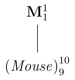
Figure 2.4: Experiment structure of enzyme levels from ten randomly sampled mice.

The number of parameters associated with each granularity are given as a superscript (one population mean and ten residuals); the subscript gives the number of independent parameters. While there are ten residuals, there are only nine degrees of freedom for their values, since knowing nine residuals and the population mean allows calculation of the value for the tenth residual. The degrees of freedom are easily calculated from the diagram: take the number of parameters (the superscript) of each factor and subtract the degrees of freedom of every factor above it.

Since (Mouse) subdivides the partition of M into a finer partition of the data, we say that (Mouse) is nested in M.

Our task is now three-fold: (i) provide an estimate of the expected population enzyme level \(\mu\) from the given data \(y_1,\dots,y_{10}\), (ii) provide an estimate of the population variance \(\sigma^2\), and (iii) quantify the uncertainty of those estimates.

The estimand is a population parameter \(\theta\) and an estimator of \(\theta\) is a function that takes data \(y_1,\dots,y_n\) as an input and returns a number that is a “good guess” of the true value of the parameter. There might be several sensible estimators for a given parameter, and statistical theory and assumptions on the data usually provide insight into which estimator is most appropriate.

We denote an estimator of a parameter \(\theta\) by \(\hat{\theta}\) and sometimes use \(\hat{\theta}_n\) to emphasize its dependence on the sample size. The estimate is the value of \(\hat{\theta}\) that results from a specific set of data. Standard statistical theory provides us with methods for constructing estimators, such as least squares, which requires few assumptions, and maximum likelihood, which requires postulating the full distribution of the data but can then better leverage them. Since the data are random, so is the estimate, and the estimator is therefore a random variable with an expectation and a variance.

2.3.1 Properties of Estimators

The bias of an estimator is the difference between its expectation and the true value of the parameter: \[ \text{bias}\left(\hat{\theta}\right) = \mathbb{E}\left(\hat{\theta}\right) - \theta = \mathbb{E}\left(\hat{\theta}-\theta\right)\;. \] We call an estimator unbiased or accurate if \(\text{bias}(\hat{\theta})=0\). Then, some realizations of our data will yield estimates that are larger than the true value, others will yield lower ones, but our estimator returns the correct parameter value on average. In contrast, a biased or inaccurate estimator systematically over- or underestimates the true parameter value (Figure 2.5).

While it is often difficult to work out the distribution of an arbitrary estimator, the distribution of an estimator derived from the maximum likelihood principle tends to a normal distribution for large sample sizes such that \[ \frac{\hat{\theta}-\theta}{\text{sd}(\hat{\theta})}\sim N(0,1)\quad\text{for $n\to\infty$} \] for an unbiased maximum likelihood estimator.

An estimator is consistent if the estimates approach the true value of the parameter when increasing the sample size indefinitely.

2.3.2 Estimators of Expectation and Variance

We now consider estimators for the mean and variance, as well as covariance and correlations as concrete examples. These estimators form the basis for more complex estimation problems that we encounter later on. We look at properties like bias and consistency in more detail to illuminate these concepts with simple examples.

The most common estimator for the expectation \(\mu\) is the arithmetic mean \[ \hat{\mu} = \bar{y} = \frac{1}{n}\sum_{i=1}^n y_i\;. \]

Our previous calculations show that \[ \mathbb{E}(\hat{\mu}) = \mathbb{E}\left(\frac{1}{n}\sum_{i=1}^n y_i\right)=\mu\;, \] and hence this estimator is unbiased.

From the data in Table 2.1, for example, we find the estimate \(\hat{\mu}=\) 10.32 for a parameter value of \(\mu=\) 10.

Similarly, the maximum likelihood estimator for the variance is \[ \dot{\sigma}^2 = \frac{1}{n}\sum_{i=1}^n (y_i-\mu)^2\;, \] but we would need \(\mu\) to calculate it. In order to make this estimator operational, we plug in the estimator \(\hat{\mu}\) instead of \(\mu\), which gives the estimator \[ \hat{\dot{\sigma}}^2 = \frac{1}{n}\sum_{i=1}^n (y_i-\hat{\mu})^2\;. \] This estimator is biased, as we easily verify: \[\begin{align*} \mathbb{E}(\hat{\dot{\sigma}}^2) &= \mathbb{E}\left(\frac{1}{n}\sum_{i=1}^n(y_i-\hat{\mu})^2\right) = \mathbb{E}\left(\frac{1}{n}\sum_{i=1}^n((y_i-\mu)-(\hat{\mu}-\mu))^2\right) \\ &= \frac{1}{n}\sum_{i=1}^n\left(\mathbb{E}((y_i-\mu)^2) \,-\, 2\cdot\mathbb{E}\left((y_i-\mu)(\hat{\mu}-\mu)\right) \,+\, \mathbb{E}((\hat{\mu}-\mu)^2)\right) \\ &= \frac{1}{n}\sum_{i=1}^n\left(\sigma^2-2\text{Cov}(y_i,\hat{\mu})+\frac{\sigma^2}{n}\right) = \frac{1}{n}\sum_{i=1}^n\left(\sigma^2-2\frac{\sigma^2}{n}+\frac{\sigma^2}{n}\right) \\ &= \left(\frac{n-1}{n}\right)\cdot\sigma^2 < \sigma^2\;. \end{align*}\] Hence, this estimator systematically underestimates the true variance. The bias decreases with increasing sample size, as \((n-1)/n\) approaches one for large \(n\).

Moreover, the bias is known and can be explicitly calculated in advance, because it only depends on the sample size \(n\) and not on the data \(y_i\). We can therefore remedy this bias simply by multiplying the estimator with \(\frac{n}{n-1}\) and thus arrive at an unbiased estimator for the variance \[ \hat{\sigma}^2 = \frac{n}{n-1}\hat{\dot{\sigma}}^2 = \frac{1}{n-1}\sum_{i=1}^n (y_i-\hat{\mu})^2\;. \] The resulting denominator \(n-1\) corresponds exactly to the degrees of freedom for the residuals in the diagram (Fig. 2.4).

An estimator for the standard deviation \(\sigma\) is \(\hat{\sigma}=\sqrt{\hat{\sigma}^2}\); this estimator is biased and no unbiased estimator for \(\sigma\) exists.

For our example, we find that the biased estimator is \(\hat{\dot{\sigma}}^2=\) 3.39 and the unbiased estimator is \(\hat{\sigma}^2=\) 3.77 (for \(\sigma^2=\) 2); the estimate of the standard deviation is then \(\hat{\sigma}=\) 1.94 (for \(\sigma=\) 1.41).

With the same arguments, we find that \[ \widehat{\text{Cov}}(X,Y) = \frac{1}{n-1}\sum_{i=1}^n\left((x_i-\hat{\mu}_X)\cdot(y_i-\hat{\mu}_Y)\right) \] is an estimator of the covariance \(\text{Cov}(X,Y)\) of two random variables \(X\) and \(Y\) with means \(\mu_X\) and \(\mu_Y\), based on \(n\) sampled pairs \((x_1,y_1),\dots,(x_n,y_n)\).

Combining this with the estimates of the standard deviations yields an estimator for the correlation \(\rho\) of \[ \hat{\rho} = \frac{\widehat{\text{Cov}}(X,Y)}{\widehat{\text{sd}}(X)\cdot\widehat{\text{sd}}(Y)}\;. \]

For our two-sample example, we find a covariance between first and second sample of \(\widehat{\text{Cov}}(Y_{i,1},Y_{i,2})=\) 3.47 and thus a very high correlation of \(\hat{\rho}=\) 0.99.

2.3.3 Standard Error and Precision

Since an estimator \(\hat{\theta}\) is a random variable, it has a variance \(\text{Var}(\hat{\theta})\), which quantifies the dispersion around its mean. Its standard deviation \(\text{sd}(\hat{\theta})\) is called the standard error of the estimator and denoted \(\text{se}(\hat{\theta})\); its reciprocal \(1/\text{se}(\hat{\theta})\) is the precision.

The distribution of an estimator not only depends on the distribution of the data, but also on the size \(n\) of the sample. Larger samples result in lower dispersion, and the standard error thus decreases with increasing sample size.

For example, the estimator \(\hat{\mu}\) has variance \(\text{Var}(\hat{\mu})=\sigma^2/n\) and its standard error \[ \text{se}(\hat{\mu})=\sigma/\sqrt{n} \] decreases with rate \(1/\sqrt{n}\) when increasing the sample size \(n\). The estimator is therefore consistent and concentrates around the true value with increasing sample size. For doubling its precision, we require four times the amount of data, and to get one more decimal place precise, a hundred-fold. We estimate the standard error by plugging in an estimate of \(\sigma^2\): \[ \widehat{\text{se}}(\hat{\mu})=\hat{\sigma}/\sqrt{n}\;. \] For our example, we find that \(\widehat{\text{se}}(\hat{\mu})=\) 0.61 and the standard error is only about 6% of the estimated expectation \(\hat{\mu}=\) 10.32, indicating high relative precision.

For normally distributed data, the ratio \[ \frac{\hat{\sigma}^2}{\sigma^2} = \frac{1}{n}\sum_{i=1}^n \left(\frac{y_i-\mu}{\sigma}\right)^2 \] has a \(\chi^2\)-distribution. To compensate for the larger uncertainty when using an estimate \(\hat{\mu}\) instead of the true value, we need to adjust the degrees of freedom and arrive at the distribution of the variance estimator \(\hat{\sigma}^2\): \[ \frac{(n-1)\hat{\sigma}^2}{\sigma^2}\sim\chi^2_{n-1}\;. \] This distribution has variance \(2(n-1)\), and from it we find the variance of the estimator to be \[ 2(n-1)=\text{Var}\left(\frac{(n-1)\hat{\sigma}^2}{\sigma^2}\right)=\frac{(n-1)^2}{\sigma^4}\text{Var}(\hat{\sigma}^2) \iff \text{Var}(\hat{\sigma}^2)=\frac{2}{n-1}\sigma^4\;. \] Hence, \(\text{se}(\hat{\sigma}^2)=\sqrt{2/(n-1)}\sigma^2\), the estimator is consistent, and doubling the precision again requires about four times as much data. The standard error now depends on the true parameter value \(\sigma^2\), and larger variances are more difficult to estimate precisely. For our example, we find that the variance estimate \(\hat{\sigma}^2=\) 3.77 has an estimated standard error of \(\widehat{\text{se}}(\hat{\sigma}^2)=\) 1.78. This is an example of an accurate (unbiased) yet imprecise estimator.

Indeed, the precision and accuracy of an estimator are complementary properties as illustrated in Figure 2.5: the precision describes the dispersion of estimates around the expected value while accuracy describes the systematic deviation between expectation and true value. Estimates might cluster very closely around a single value, indicating high precision, yet estimates might still be incorrect for a biased estimator when this single value is not the true parameter value.

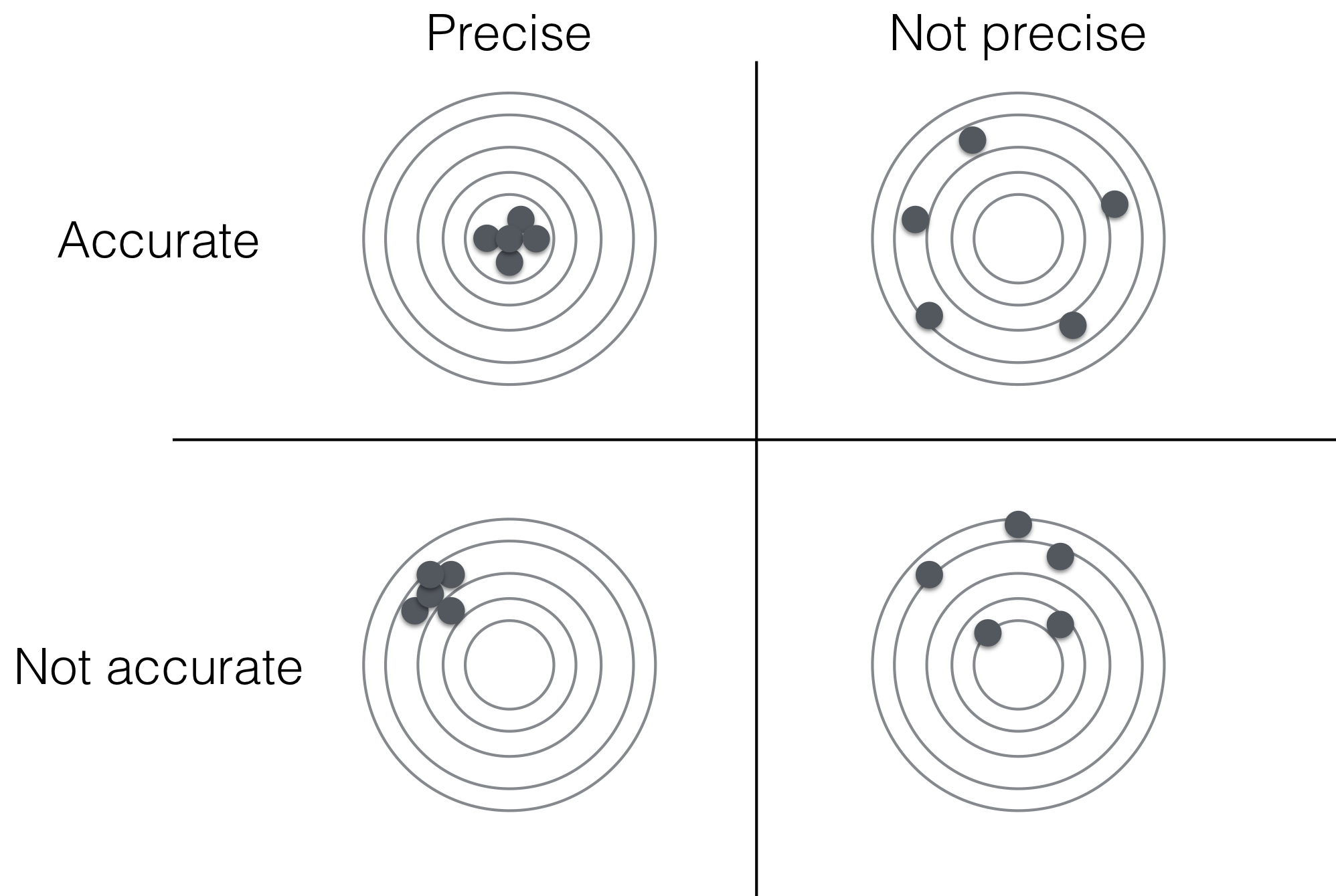
Figure 2.5: Accuracy and precision of an estimator.

2.3.4 Confidence Intervals

The estimators for expectation and variance are examples of point estimators and provide a single number as the “best guess” of the true parameter from the data. The standard error quantifies the uncertainty of a point estimate: an estimate of the average enzyme level based on one hundred mice is more precise than an estimate based on only two mice.

A confidence interval of a parameter \(\theta\) is another way for quantifying the uncertainty that additionally takes account of the full distribution of the estimator. The interval contains all values of the parameter that are compatible with the observed data up to a specified degree. The \((1-\alpha)\)-confidence interval of an estimator \(\hat{\theta}\) is an interval \([a(\hat{\theta}),b(\hat{\theta})]\) such that \[ \mathbb{P}\left(a(\hat{\theta})\leq \theta \leq b(\hat{\theta})\right) = 1-\alpha\;. \] We call the values \(a(\hat{\theta})\) and \(b(\hat{\theta})\) the lower and upper confidence limit, respectively, and abbreviate them as LCL and UCL. The confidence level \(1-\alpha\) quantifies the degree of being ‘compatible with the data.’ The higher the confidence level (the lower \(\alpha\)), the wider the interval, until a 100%-confidence interval includes all possible values of the parameter and becomes useless.

While not strictly required, we always choose the confidence limits \(a\) and \(b\) such that the left and right tail each cover half of the required confidence level. This provides the shortest possible confidence interval.

The confidence interval equation is a probability statement about a random interval covering \(\theta\) and not a statement about the probability that \(\theta\) is contained in a given interval. For example, it is incorrect to say that, having computed a 95%-confidence interval of \([-2, 2]\), the true population parameter has a 95% probability of being larger than \(-2\) and smaller than \(+2\). Such a statement would be nonsensical, because any given interval either contains the true value (which is a fixed number) or it does not, and there is no probability attached to this.

One correct interpretation is that the proportion of intervals containing the correct value \(\theta\) is \((1-\alpha)\) under repeated sampling and estimation. This interpretation is helpful in contexts like quality control, where the ‘same’ experiment is done repeatedly and there is thus a direct interest in the proportion of intervals containing the true value. For most biological experiments, we do not anticipate repeating them over and over again. Here, an equivalent interpretation is that our specific confidence interval, computed from the data of our experiment, has a \((1-\alpha)\) probability to contain the correct parameter value.

For computing a confidence interval, we need to derive the distribution of the estimator; for maximum likelihood estimators this distribution is normal for large sample sizes, and \[ \frac{\theta-\hat{\theta}}{\text{se}(\hat{\theta})} \sim N(0,1)\;, \] and therefore \[ z_{\alpha/2}\leq \frac{\theta-\hat{\theta}}{\text{se}(\hat{\theta})} \leq z_{1-\alpha/2} \quad\text{with probability}\quad 1-\alpha\;, \] where \(z_\alpha\) is the \(\alpha\)-quantile of the standard normal distribution. Rearranging terms yields the well-known asymptotic confidence interval for an unbiased maximum likelihood estimator \[ \left[ \hat{\theta}+z_{\alpha/2}\cdot\text{se}(\hat{\theta}),\; \hat{\theta}+z_{1-\alpha/2}\cdot\text{se}(\hat{\theta}) \right]\;. \] For some standard estimators, the exact distribution might not be normal, but is nevertheless known. If the distribution is unknown or difficult to compute, we can use computational methods such as the bootstrap to find an approximate confidence interval.

2.3.4.1 Confidence Interval for Mean Estimate

For normally distributed data \(y_i\sim N(\mu,\sigma^2)\), we know that \[ \frac{\hat{\mu}-\mu}{\sigma/\sqrt{n}}\sim N(0,1) \quad\text{and}\quad \frac{\hat{\mu}-\mu}{\hat{\sigma}/\sqrt{n}}\sim t_{n-1} \;. \] The normal distribution is appropriate if the variance is known or if the sample size \(n\) is large.

We then construct a \((1-\alpha)\)-confidence interval based on the normal distribution: \[ \left[ \hat{\mu}+z_{\alpha/2}\cdot \sigma / \sqrt{n},\; \hat{\mu}+z_{1-\alpha/2}\cdot \sigma / \sqrt{n} \right] \,=\, \hat{\mu}\pm z_{\alpha/2}\cdot \sigma / \sqrt{n}\;. \] The equality holds because \(z_{\alpha/2}=-z_{1-\alpha/2}\). For small sample sizes \(n\), we need to take account of the additional uncertainty from replacing \(\sigma\) by \(\hat{\sigma}\). The exact confidence interval of \(\mu\) is then \[ \hat{\mu}\pm t_{\alpha/2,\,n-1}\cdot\widehat{\text{se}}(\hat{\mu}) \,=\, \hat{\mu}\pm t_{\alpha/2,\,n-1}\cdot \hat{\sigma}/\sqrt{n}\;. \]

For our data, the 95%-confidence interval based on the normal approximation is [9.11, 11.52] and the interval based on the \(t\)-distribution [8.93, 11.71] is wider. For larger samples sizes \(n\), the difference between the two intervals quickly becomes negligible.

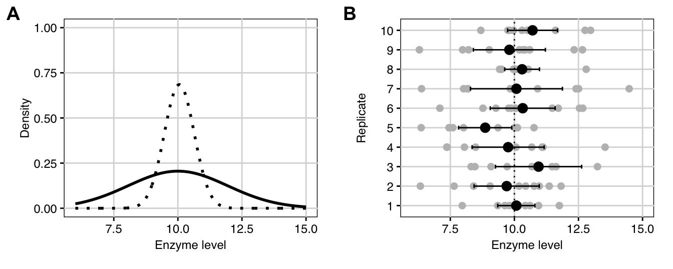
Figure 2.6: A: Distribution of enzyme levels in population (solid) and of average (dotted); B: Levels measured for ten replicates of ten randomly sampled mice each (grey points) with estimated mean for each replicate (black points) and their 95% confidence intervals (black lines) compared to true mean (dotted line).

To further illustrate confidence intervals, we return to our enzyme level example. The true \(N(10,2)\)-density of enzyme levels is shown in Figure 2.6A (solid line) and the \(N(10,2/10)\)-density of the estimator of the expectation based on ten samples is shown as a dotted line. The rows of Figure 2.6B are the enzyme levels of ten replicates of ten randomly sampled mice as grey points, with the true average \(\mu=\) 10 shown as a vertical dotted line. The resulting estimates of the expectation and their 95%-confidence intervals are given as black points and lines, respectively. The ten estimates vary much less than the actual measurements and fall both above and below the true expectation. Since the confidence intervals are based on the random samples, they have different lower and upper confidence limits and different lengths. For a confidence limit of 95% we expect that 1 out of 20 confidence intervals does not to cover the true value on average; an example is the interval of replicate five that covers only values below the true expectation.

2.3.4.2 Confidence Interval for Variance Estimate

For the variance estimator, recall that \((n-1)\hat{\sigma}^2/\sigma^2\) has a \(\chi^2\)-distribution. It follows that \[ \chi^2_{\alpha/2,\,n} \leq \frac{(n-1)\hat{\sigma}^2}{\sigma^2}\leq \chi^2_{ 1-\alpha/2,\,n-1}\quad\text{with probability $1-\alpha$}\;, \] where \(\chi^2_{\alpha,\,n}\) is the \(\alpha\)-quantile of a \(\chi^2\)-distribution with \(n\) degrees of freedom. Rearranging terms, we find the \((1-\alpha)\)-confidence interval \[ \frac{(n-1)\hat{\sigma}^2}{\chi^2_{1-\alpha/2,\,n-1}} \leq \sigma^2 \leq \frac{(n-1)\hat{\sigma}^2}{\chi^2_{\alpha/2,\,n-1}}\;. \] This interval does not simplify to the form \(\hat{\theta}\pm q_\alpha\cdot \text{se}\), because the \(\chi^2\)-distribution is not symmetric and \(\chi^2_{\alpha,\,n}\not=-\chi^2_{1-\alpha,\,n}\).

For our example, we estimate the population variance as \(\hat{\sigma}^2=\) 3.77 (for a true value of \(\sigma^2=\) 2). With \(n-1=\) 9 degrees of freedom, the two quantiles for a 95%-confidence interval are \(\chi^2_{0.025,\,9}=\) 2.7 and \(\chi^2_{0.975,\,9}=\) 19.02, leading to an interval of [1.78, 12.56]. The interval covers the true value, but its width indicates that our variance estimate is quite imprecise. A confidence interval for the standard deviation \(\sigma\) is calculated by taking square-roots of the lower and upper confidence limits of the variance. This yields a 95%-confidence interval of [1.34, 3.54] for our estimate \(\hat{\sigma}=\) 1.94 (true value of \(\sigma=\) 1.41).

2.3.5 Estimation for Comparing Two Samples

Commonly, we are interested in comparing properties of two different samples to determine if there are detectable differences between their distributions. For example, if we always used a sample preparation kit of vendor A for our enzyme level measurements, but vendor B now also has a (maybe cheaper) kit available, we may want to establish if the two kits yield similar results. For this example, we are specifically interested in establishing if there is a systematic difference between measurements based on kit A compared to kit B or if measurements from one kit are more dispersed than from the other.

We denote by \(\mu_A, \mu_B\) the expectations and by \(\sigma^2_A, \sigma^2_B\) the variances of the enzyme levels \(y_{i,A}\) and \(y_{i,B}\) measured by kit A and B, respectively. Our interest focuses on two effect sizes: we measure the systematic difference between the kits by the difference \(\Delta=\mu_A-\mu_B\) of their expected values, and we measure the difference in variances by their proportion \(\Pi=\sigma_A^2/\sigma_B^2\). Since we already have ten measurements with our standard kit A, our proposed experiment is to select another ten mice and measure their levels using kit B. This results in the data shown in Table 2.3, whose first row is identical to our previous data.

Our goal is to establish an estimate of the difference in means and the proportion of variances, and to calculate confidence intervals for these estimates.

Table 2.3: Measured enzyme levels for 20 mice, measured by kits from two vendors A and B.

A	8.96	8.95	11.37	12.63	11.38	8.36	6.87	12.35	10.32	11.99
B	12.68	11.37	12.00	9.81	10.35	11.76	9.01	10.83	8.76	9.99

The logical structure of the experiment is shown in the diagram in Figure 2.7.

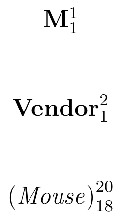
Figure 2.7: Experiment for estimating the difference in enzyme levels by randomly assigning 10 mice each to two vendors.

The data from this experiment are described by the \(\mu=(\mu_A+\mu_B)/2\), given by the factor M; this is the ‘best guess’ for the value of any datum \(y_{ij}\) if nothing else is known. If we know which vendor was assigned to the datum, a better ‘guess’ is the corresponding mean \(\mu_A\) or \(\mu_B\). The factor Vendor is associated with the two differences \(\mu_A-\mu\) and \(\mu_B-\mu\). Since we can calculate \(\mu_A\), say, from \(\mu\) and \(\mu_B\), the degrees of freedom for this factor are one. Finally, the next finer partition of the data is into the individual observations; their \(2\cdot 10\) residuals \(e_{ij}=y_{ij}-\mu_i\) are associated with the factor (Mouse), and only 18 of the residuals are independent given the two group means. In this diagram, (Mouse) is nested in Vendor and Vendor is nested in M since each factor further subdivides the partition of the factor above. This implies that (Mouse) is also nested in M.

The diagram corresponds to the model \[ y_{ij} = \mu + \delta_i + e_{ij} \] for the data, where \(\delta_i=\mu-\mu_i\) are the deviations from grand mean to group mean and \(\mu_A=\mu+\delta_A\) and \(\mu_B=\mu+\delta_B\). The three parameters \(\mu\), \(\delta_A\) and \(\delta_B\) are unknown but fixed quantities, while the \(e_{ij}\) are random and interest focuses on their variance \(\sigma^2\).

2.3.5.1 Proportion of Variances

For two normally distributed samples of size \(n\) and \(m\), respectively, we estimate the proportion of variances as \(\hat{\Pi}=\hat{\sigma}^2_A/\hat{\sigma}^2_B\). We derive a confidence interval for this estimator by noting that \((n-1)\hat{\sigma}_A^2/\sigma_A^2\sim\chi^2_{n-1}\) and \((m-1)\hat{\sigma}_B^2/\sigma_B^2\sim\chi^2_{m-1}\). Then, \[ \frac{\frac{(n-1)\hat{\sigma}_A^2}{\sigma_A^2}/(n-1)} {\frac{(m-1)\hat{\sigma}_B^2}{\sigma_B^2}/(m-1)} =\frac{\hat{\sigma}_A^2/\sigma_A^2}{\hat{\sigma}_B^2/\sigma_B^2} =\frac{\hat{\Pi}}{\Pi}\sim F_{n-1,m-1} \] has an \(F\)-distribution with \(n-1\) numerator and \(m-1\) denominator degrees of freedom. A \((1-\alpha)\)-confidence interval for \(\Pi\) is therefore \[ \left[\frac{\hat{\Pi}}{F_{1-\alpha/2,\,n-1,\, m-1}},\,\frac{\hat{\Pi}}{F_{\alpha/2,\,n-1,\, m-1}}\right]\;. \] For our example, we find the two individual estimates \(\hat{\sigma}^2_A=\) 3.77 and \(\hat{\sigma}^2_B=\) 1.69 and an estimated proportion \(\hat{\Pi}=\) 2.23. This yields a 95%-confidence interval for \(\hat{\Pi}\) of [0.55, 8.98], which contains the ratio of one (meaning equal variances) and values below and above one. Hence, given the data, we have no evidence that the two true variances are substantially different, even though their estimates differ by a factor of more than 2.

2.3.5.2 Difference in Means of Independent Samples

We estimate the systematic difference \(\Delta\) between the two kits as \[ \hat{\Delta}=\widehat{\mu_A-\mu_B} = \hat{\mu}_A-\hat{\mu}_B\;, \] the difference between the estimates of the respective expected enzyme levels.

For the example, we estimate the two average enzyme levels as \(\hat{\mu}_A=\) 10.32 and \(\hat{\mu}_B=\) 10.66 and the difference as \(\hat{\Delta}=-0.34\). The estimated difference is not exactly zero, but this might be explainable by measurement error or the natural variation of enzyme levels between mice.

We take account of the uncertainty by calculating the standard error and a 95%-confidence interval for \(\hat{\Delta}\). The lower and upper confidence limits then provide information about a potential systematic difference: if the upper limit is below zero, then only negative differences are compatible with the data, and we can conclude that measurements of kit A are systematically lower than measurements of kit B. Conversely, a lower limit above zero indicates kit A yielding systematically higher values than kit B. If zero is contained in the confidence interval, we cannot determine the direction of a potential difference, and it is also plausible that no difference exists.

We already established that the data provides no evidence against the assumption that the two variances are equal. We therefore assume a common variance \(\sigma^2=\sigma^2_A=\sigma^2_B\), which we estimate by the pooled variance estimate \[ \hat{\sigma}^2 = \frac{\hat{\sigma}_A^2+\hat{\sigma}_B^2}{2}\;. \] For our our data, \(\hat{\sigma}^2=\) 2.73 and the estimated standard deviation is \(\hat{\sigma}=\) 1.65.

Compared to this standard deviation, the estimated difference is small (about 21%). Whether such a small difference is meaningful in practice depends on the subject matter. A helpful dictum is

A difference which makes no difference is no difference at all. (attributed to William James)

To determine the confidence limits, we first need the standard error of the difference estimate. The two estimates \(\hat{\mu}_A\) and \(\hat{\mu}_B\) are based on independently selected mice, and are therefore independent. Simple application of the rules for variances then yields: \[ \text{Var}(\hat{\Delta}) = \text{Var}(\hat{\mu}_A-\hat{\mu}_B) = \text{Var}(\hat{\mu}_A)+\text{Var}(\hat{\mu}_B)=2\cdot\frac{\sigma^2}{n}\;. \] The standard error of the difference estimator is therefore \[ \text{se}(\hat{\Delta}) = \sqrt{2\cdot\frac{\sigma^2}{n}}\;, \] which yields \(\widehat{\text{se}}(\hat{\Delta})=\) 0.74. The \((1-\alpha)\)-confidence interval \[ \hat{\Delta} \pm t_{\alpha/2,\,2n-2}\cdot \widehat{\text{se}}(\hat{\Delta}) \quad=\quad(\hat{\mu}_A-\hat{\mu}_B) \pm t_{\alpha/2,\,2n-2}\cdot \sqrt{2\cdot\frac{\hat{\sigma}^2}{n}}\;. \] follows from the previous arguments.

Note that we have \(2n\) observations in total, from which we estimate the two means, resulting in \(2n-2\) degrees of freedom for the \(t\)-distribution; these are the \(18\) degrees of freedom of the factor (Mouse) in Figure 2.7.

For our data, we calculate a 95%-confidence interval of \([-1.89, 1.21]\). The confidence interval contains the value zero, and the two kits might indeed produce equivalent values. The interval also contains negative and positive values of substantial magnitude that are possibly relevant in practice. We can therefore only conclude that there is no evidence of a systematic difference between kits, but if such difference existed, it might be large enough to be practically relevant. This non-result should have been avoided with proper experimental design.

2.3.5.3 Difference in Means of Dependent Samples

We find a very different result when we address the same question using the design illustrated in Figure 1.1C, where we randomly select ten mice, draw two samples from each, and randomly assign each kit to one sample. The resulting data are given in Table 2.4.

Table 2.4: Enzyme levels for vendor A and B based on two samples from each of ten mice, one sample per vendor.

Mouse	1	2	3	4	5	6	7	8	9	10
A	9.14	9.47	11.14	12.45	10.88	8.49	7.62	13.05	9.67	11.63
B	9.19	9.70	11.12	12.62	11.50	8.99	7.54	13.38	10.94	12.28

The Hasse diagram for this experiment is shown in Figure 2.8A. The two factors (Mouse) and Vendor are now crossed and written next to each other. Each sample corresponds to a combination of one mouse and one vendor, and is nested in both. Since the mice are randomly selected, their average responses are also random.

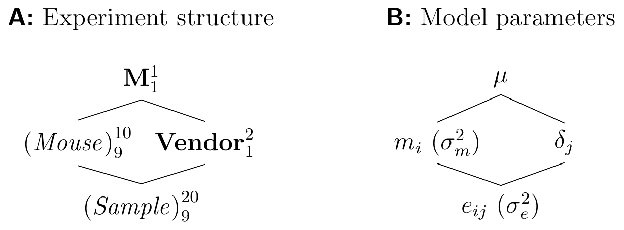
Figure 2.8: Paired design for estimating average enzyme level difference: 10 mice, each vendor assigned to one of two samples per mouse.

The two observations from mouse \(i\) are \[ y_{iA} = \mu + \delta_A + m_i + e_{iA}\quad\text{and}\quad y_{iB} = \mu + \delta_B + m_i + e_{iB}\;, \] where \(\text{Var}(m_i)=\sigma_m^2\), and \(\text{Var}(e_{ij})=\sigma_e^2\). The parameters \(\delta_A=-\delta_B\) are the treatment effects. The expected response with kit A is then \(\mu+\delta_A\), and the variance of any observation is \(\text{Var}(y_{ij})=\sigma_m^2+\sigma_e^2\). This model corresponds directly to the diagram, as shown in Figure 2.8B. We estimate the average enzyme level from kit A as \(\hat{\mu}_A=\sum_{i=1}^n y_{iA}/n\) and from kit B as \(\hat{\mu}_B=\sum_{i=1}^n y_{iB}/n\). An estimate of their difference \(\Delta'=\mu_A-\mu_B\) is then \[ \hat{\Delta}'=\frac{1}{n}\sum_{i=1}^n (y_{i,A}-y_{i,B})=\frac{1}{n}\sum_{i=1}^n y_{i,A}-\frac{1}{n}\sum_{i=1}^n y_{i,B}=\hat{\mu}_A-\hat{\mu}_B\;. \] This is the same estimator as for two independent samples, and yields a similar estimated difference of \(\hat{\Delta}'=\) -0.37 for our example.

The variance of this estimator is very different, however, due to the correlation between each pair of samples: \[ \text{Var}(\hat{\Delta}')=\text{Var}(\hat{\mu}_A)+\text{Var}(\hat{\mu}_B)-2\cdot\text{Cov}(\hat{\mu}_A,\hat{\mu}_B) =2\frac{\sigma_m^2+\sigma_e^2}{n}-2\frac{\sigma_m^2}{n}=2\frac{\sigma_e^2}{n}\;. \] In other words, contrasting the two kits within each mouse and then averaging these differences over the ten mice eliminates the between-mouse variation \(\sigma_m^2\) from the treatment comparison.

For the data in Table 2.4, we find the two means \(\hat{\mu}_A=\) 10.35 and \(\hat{\mu}_B=\) 10.73 together with the variances \(\hat{\sigma}^2_A=\) 3.1 and \(\hat{\sigma}^2_B=\) 3.38, and a non-zero covariance of \(\widehat{\text{Cov}}=\) 3.16. The standard error of the difference estimate is then \(\widehat{\text{se}}(\hat{\Delta}')=\) 0.13, much lower than the previous standard error \(\widehat{\text{se}}(\hat{\Delta})=\) 0.74.

The \((1-\alpha)\)-confidence interval for \(\Delta'\) is \[ \hat{\Delta}'\pm t_{\alpha/2,n-1}\cdot\text{se}(\hat{\Delta}')\;, \] and is based on \(n-1=\) 9 degrees of freedom (note that we have a single sum with 10 summands, not two independent sums!). The 95%-confidence interval for our data is \([-0.66, -0.08]\) and is much narrower than the interval \([-1.89, 1.21]\) of the previous example due to the substantial increase in precision. It only contains negative values, indicating that kit A consistently yields lower values than kit B. The differences compatible with the data are small, and subject-matter considerations can help determine if such differences are practically relevant. In contrast to the previous experiment, we now arrived at a satisfactory result from which relevant conclusions can be drawn.

Standardized Effect Size for Difference

The difference \(\Delta\) is an example of a raw effect size and has the same units as the original measurements. Subject-matter knowledge often provides information about the relevance of specific effect sizes and might tell us, for example, if a difference in enzyme levels of more than 0.5 is biologically relevant.

Sometimes the raw effect size is difficult to interpret. This is a particular problem with some current measurement techniques in biology, which give measurements in arbitrary units (a.u.), making it difficult to directly compare results from two experiments. In this case, a unit-less standardized effect size might be more appropriate. A popular choice is Cohen’s \(d\), which compares the difference with the standard deviation in the population: \[ d = \frac{\mu_A-\mu_B}{\sigma} \quad\text{estimated by}\quad \hat{d} = \frac{\hat{\mu}_A-\hat{\mu}_B}{\hat{\sigma}}\;. \] It is a unit-less effect size that measures the difference as a multiple of the standard deviation. If \(|d|=1\), then the two means are one standard deviation apart. In the original literature, Cohen suggests that \(|d|<0.2\) should be considered a small effect, \(0.2<|d|<0.5\) a medium-sized effect, and \(0.5<|d|<0.8\) a large effect (Cohen 1988), but such definitive categorization should not be taken too literally.

For our example, we calculate \(\hat{d}=\) \(-0.21\), a difference of 21% of a standard deviation, indicating a small-to-medium effect size. The exact confidence interval for \(\hat{d}\) is based on a noncentral \(t\)-distribution and cannot be given in closed form (cf. Section 2.5). For large enough sample size, we can use a normal confidence interval \(\hat{d}\pm z_{\alpha/2}\cdot\widehat{\text{se}}(\hat{d})\) based on an approximation of the standard error (Hedges and Olkin 1985): \[ \widehat{\text{se}}(\hat{d}) = \sqrt{ \frac{n_A+n_B}{n_A\cdot n_B}+\frac{\hat{d}^2}{2\cdot(n_A+n_B)} }\;, \] where \(n_A\) and \(n_B\) are the respective sample sizes for the two groups. For our example, this yields an approximate 95%-confidence interval of \([-1.08, 0.67]\).

2.4 Testing Hypotheses

The underlying question in our kit vendor example is whether the statement \(\mu_A=\mu_B\) about the underlying parameters is true or not. We argued that the data would not support this statement if the confidence interval of \(\Delta\) lies completely above or below zero, excluding \(\Delta=0\) as a plausible difference. Significance testing is an equivalent way of using the observations for evaluating the evidence in favor or against a specific null hypothesis, such as \[ H_0: \mu_A=\mu_B \quad\text{or equivalently}\quad H_0: \Delta=0\;. \] The null hypothesis is a statement about the true value of one or more parameters.

2.4.1 The Logic of Falsification

Testing hypotheses follows a logic closely related to that of scientific research in general: we start from a scientific conjecture or theory to explain a phenomenon. From the theory, we derive observable consequences (or predictions) that we test in an experiment. If the predicted consequences are in substantial disagreement with those experimentally observed, then the theory is deemed implausible and is rejected or falsified. If, on the other hand, prediction and observation are in agreement, then the experiment failed to reject the theory. However, this does not mean that the theory is proven or verified since the agreement might be due to chance, the experiment not specific enough, or the data too noisy to provide sufficient evidence against the theory:

Absence of evidence is not evidence of absence.

It is instructive to explicitly write down this logic more formally. The correctness of the conjecture \(C\) implies the correctness of the prediction \(P\): \[ C \text{ true}\implies P\text{ true}\;. \] We say \(C\) is sufficient for \(P\). We now perform an experiment to determine if \(P\) is true. If the experiment supports \(P\), we did not gain much, since we cannot invert the implication and conclude that the conjecture \(C\) must also be true. Many other possible conditions might lead to the predicted outcome that have nothing to do with our conjecture.

However, if the experiment shows the prediction \(P\) to be false, then we can invoke the modus tollens \[ P \text{ false} \implies C\text{ false} \] and conclude that \(C\) cannot be true. We say \(P\) is necessary for \(C\). There is thus an asymmetry in the relation of “\(P\) is true” and “\(P\) is false” towards the correctness of \(C\), and we can falsify a theory (at least in principle), but never fully verify it. The philosopher Karl Popper argued that falsification is a cornerstone of science and falsifiability (in principle) of conjectures separates a scientific theory from a non-scientific one (Popper 1959).

Statistical testing of hypotheses follows a similar logic, but adds a probabilistic argument to quantify the (dis-)agreement between hypothesis and observation. The data may provide evidence to reject the null hypothesis, but can never provide evidence for accepting the null hypothesis. We therefore formulate a null hypothesis for the ‘undesired’ outcome such that if we don’t reject it, nothing is gained and we don’t have any clue from the data how to proceed in our investigation. If the data provides evidence to reject the hypothesis, however, we can reasonably exclude it as a possible explanation of the observed data.

To appraise the evidence that our data provides against the null hypothesis, we need to take the random variation in the data into account. Instead of a yes/no answer, we can then only argue that “if the hypothesis is true, then it is (un-)likely that data like ours are observed.” This is precisely the argument from the hypothesis to the observable consequences, but with a probabilistic twist.

2.4.2 The \(t\)-test

For our example, we know that if the true difference \(\Delta\) is zero, then the estimated difference \(\hat{\Delta}\) divided by its standard error has a \(t\)-distribution. This motivates the well-known t-statistic \[\begin{equation} T = \frac{\hat{\Delta}}{\widehat{\text{se}}(\hat{\Delta})} = \frac{\hat{\Delta}}{\sqrt{2\cdot \hat{\sigma}^2/n}} \sim t_{2n-2}\;. \tag{2.1} \end{equation}\]

Thus, our conjecture is “the null hypothesis is true and \(\Delta=0\)” from which we derive the prediction “the observed test statistic \(T\) based on the two sample averages follows a \(t\)-distribution with \(2n-2\) degrees of freedom.”

For our data, we compute a \(t\)-statistic of \(t=-0.46\), based on the two means 10.32 for vendor A, 10.66 for vendor B, their difference \(\hat{\Delta}=-0.34\), and the resulting standard error of 0.74 of the difference on 18 degrees of freedom. The estimated difference in means is expressed by \(t\) as about 46% of a standard error, and the sign of \(t\) indicates that measurements with kit A might be lower than with kit B.

The test statistic remains the same for the cases of paired data as in Figure 1.1C, with standard error calculated as in Section 2.3.5.3; this is known as a paired \(t\)-test.

2.4.3 \(p\)-values and Statistical Significance

\(p\)-values

If we assume that the hypothesis \(H_0\) is true, we can compute the probability that our test statistic \(T\) exceeds any given value in either direction using its known distribution. Calculating this probability for the observed value \(t\) provides us with a quantitative measure of the evidence that the data provide against the hypothesis. This probability is called the \(p\)-value \[ p = \mathbb{P}(|T|\geq |t|\,|\, H_0\text{ true})\;. \] Because our test statistic is random (it is a function of the random samples), the \(p\)-value is also a random variable. If the null hypothesis is true, then \(p\) has a uniform distribution between \(0\) and \(1\).

For our example, we compute a \(p\)-value of 0.65, and we expect a \(t\)-statistic that deviates from zero by 0.46 or more in either direction in 65 out of 100 cases whenever the null hypothesis is true. We conclude that based on the variation in the data and the sample size, observing a difference of at least this magnitude is very likely and there is no evidence against the null hypothesis.

A small \(p\)-value is considered indicative of \(H_0\) being false, since it is unlikely that the observed (or larger) value of the test statistic would occur if the hypothesis were true. This leads to a dichotomy of explanations for small \(p\)-values: either the data led to the large value just by chance, or the null hypothesis is wrong and the test statistic does not follow the predicted distribution. On the other hand, a large \(p\)-value might occur either because \(H_0\) is true or because \(H_0\) is false but our data did not yield sufficient information to detect the true difference in means.

We may still decide to ignore a large \(p\)-value and nevertheless move ahead and assume that \(H_0\) is wrong; but the argument for doing so cannot rest on the single experimental result and its statistical analysis, but must include external arguments such as subject-matter considerations (e.g., about plausible effects) or outcomes of related experiments.

If possible, we should always combine an argument based on a \(p\)-value with the observed effect size: a small \(p\)-value (indicating that the effect found can be distinguished from noise) is only meaningful if the observed effect size has a practically relevant magnitude. Even a large effect size might yield a large \(p\)-value if the sample size is small and the variation in the data is large. In our case, the estimated difference of \(\hat{\Delta}=-0.34\) is small compared to the standard error \(\widehat{\text{se}}(\hat{\Delta})=\) 0.74 and cannot be distinguished from random fluctuation. That our test does not provide evidence for a difference, however, does not mean it does not exist.

Conversely, a low \(p\)-value means that we were able to distinguish the observed difference from a random fluctuation, but the detected difference might have a tiny and irrelevant effect size if random variation is low or sample size large. However, this provides only one (crucial) piece of the argument why we suggest a particular interpretation and rule out others. It does not excuse us from proposing a reasonable interpretation of the whole investigation and other experimental data.

Statistical Significance

We sometimes use a pre-defined significance level \(\alpha\) against which we compare the \(p\)-value. If \(p<\alpha\), then we consider the \(p\)-value low enough to reject the null-hypothesis and we call the test statistically significant. The hypothesis is not rejected otherwise, a result called not significant. The level \(\alpha\) codifies our judgement of what constitutes a ‘just by chance’ event, and is the probability to incorrectly reject a true null hypothesis. There is no theoretical justification for any choice of this threshold, but for as much historical as practical reasons, values of \(\alpha=5\%\) or \(\alpha=1\%\) are commonly used. In our example, \(p=0.65\) far exceeds both thresholds and the test outcome is thus deemed not significant.

All cautionary notes for \(p\)-values apply to significance statements as well. In particular, just because a test found a significant difference does not imply that the difference is practically meaningful:

Statistical significance does not imply scientific significance.

Moreover, the \(p\)-value or a statement of significance concern a single experiment, but a single significant result is not enough to establish scientific significance of a result:

In order to assert that a natural phenomenon is experimentally demonstrable we need, not an isolated record, but a reliable method of procedure. In relation to the test of significance, we may say that a phenomenon is experimentally demonstrable when we know how to conduct an experiment which will rarely fail to give us a statistically significant result. (Fisher 1971)

as R. A. Fisher rightly insisted.

Instead of comparing the \(p\)-value with the significance level, we can equivalently compare the observed test statistic \(t\) with the corresponding quantiles of the null-distribution. We then reject the null hypothesis if \(T<t_{\alpha/2,\,2n-2}\) (kit A lower) or \(T>t_{1-\alpha/2,\, 2n-2}\) (kit B lower). For our example with \(\alpha=5\%\), the thresholds are \(t_{0.025,\,18}=-2.1\) and \(t_{0.975,\,18}=2.1\). Our observed \(t\)-statistic \(t=-0.46\) lies within these thresholds and the hypothesis is not rejected.

Error Probabilities

Any statistical test has four possible outcomes under the significant / non-significant dichotomy, which we summarize in Table 2.5. A significant result leading to rejection of \(H_0\) is called a positive. If the null hypothesis is indeed false, then it is a true positive, but if the null hypothesis is indeed true, it was incorrectly rejected: a false positive or type-I error. The significance level \(\alpha\) is the probability of a false positive and by choosing a specific value, we can control the type-I error of our test. The specificity of the test is the probability \(1-\alpha\) that we correctly do not reject a true null hypothesis.

Conversely, a non-significant result is called a negative. Not rejecting a true null hypothesis is a true negative, incorrectly not rejecting a false null hypothesis is a false negative or a type-II error. The probability of a false negative test outcome is denoted by \(\beta\). The power or sensitivity of the test is the probability \(1-\beta\) that we correctly reject the null hypothesis. The larger the true effect size, the more power a test has to detect it. Power analysis allows us to determine the test parameters (most importantly, the sample size) to provide sufficient power for detecting an effect size deemed scientifically relevant.

Table 2.5: The four possible outcomes of a hypothesis test.

	\(H_0\) true	\(H_0\) false
No rejection	true negative (TN)	false negative (FN)
	specificity \(1-\alpha\)	\(\beta\)
Rejection	false positive (FP)	true positive (TP)
	\(\alpha\)	sensitivity or power \(1-\beta\)

Everything else being equal, the two error probabilities \(\alpha\) and \(\beta\) are adversaries: by lowering the significance level \(\alpha\), larger effects are required to reject the null hypothesis, which simultaneously increases the probability \(\beta\) of a false negative.

This has an important consequence: if our experiment has low power (it is underpowered), then only large effect sizes yield statistical significance. A significant \(p\)-value and a large effect size then tempt us to conclude that we reliably detected a substantial difference, even though we must expect such a result with probability \(\alpha\) in the case that no difference exists.

Under repeated application of a test with new data, \(\alpha\) and \(\beta\) are the expected frequencies—the false positive rate respectively the false negative rate—of the two types of error. This interpretation is helpful in scenarios such as quality control. On the other hand, we usually conduct only a limited number of repeated test in scientific experimentation. Here, we can interpret \(\alpha\) and \(\beta\) as quantifying the severity of a statistical test—its hypothetical capability to detect a desired difference in a planned experiment. This is helpful for planning experiments to ensure that the data generated will likely provide sufficient evidence against an incorrect scientific hypothesis.

Rejection Regions and Confidence Intervals

Instead of rejecting \(H_0\) if the test statistic \(T\) exceeds the respective \(t\)-quantiles, we can also determine the corresponding limits on the estimated difference \(\hat{\Delta}\) directly and reject if \[\begin{equation*} \hat{\Delta}< t_{\alpha/2,\,2n-2}\cdot\sqrt{2}\cdot \hat{\sigma}/\sqrt{n} \quad\text{or}\quad \hat{\Delta}> t_{1-\alpha/2,\,2n-2}\cdot\sqrt{2}\cdot \hat{\sigma}/\sqrt{n} \;. \end{equation*}\] The corresponding set of values is called the rejection region \(\mathcal{R}\) and we reject \(H_0\) whenever the observed difference \(\hat{\Delta}\) falls inside \(\mathcal{R}\). In our example, \(\mathcal{R}\) consists of the two sets \((-\infty,-1.55)\) and \((1.55,+\infty)\). Since \(\hat{\Delta}=-0.34\) does not fall into this region, we do not reject the null hypothesis.

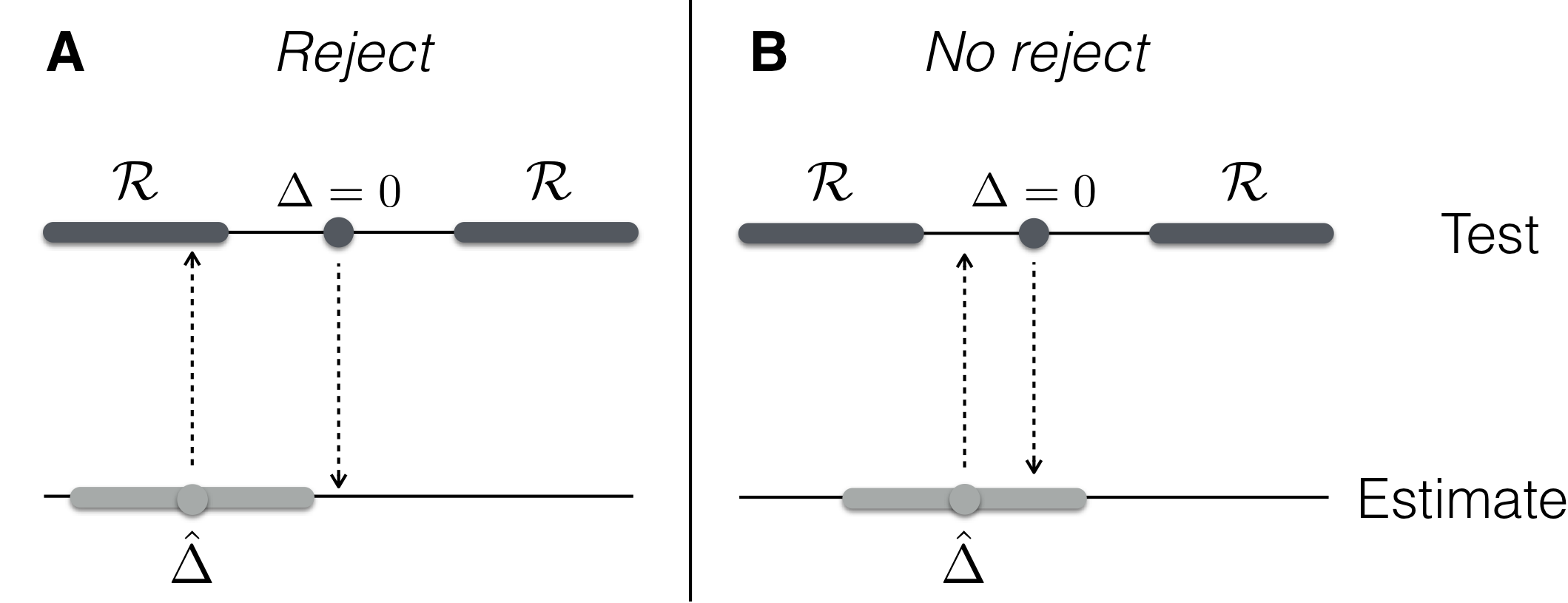
Figure 2.9: Equivalence of testing and estimation. A: Estimate inside rejection region and null value outside the confidence interval. B: Estimate outside rejection region, confidence interval contains null value. Top: null value (dark grey dots) and rejection region (dark grey shades); bottom: estimate \(\hat{\Delta}\) (light grey dots) and confidence interval (light grey shades).

There is a one-to-one correspondence between the rejection region \(\mathcal{R}\) for a significance level \(\alpha\), and the \((1-\alpha)\)-confidence interval of the estimated difference. The estimated effect \(\hat{\Delta}\) lies inside the rejection region if and only if the value 0 is outside its \((1-\alpha)\)-confidence interval. This equivalence is illustrated in Figure 2.9. In hypothesis testing, we put ourselves on the value under \(H_0\) (e.g., \(\Delta=0\)) and check if the estimated value \(\hat{\Delta}\) is so far away that it falls inside the rejection region. In estimation, we put ourselves at the estimated value \(\hat{\Delta}\) and check if the data provide no objection against the hypothesized value under \(H_0\), which then falls inside the confidence interval. Our previous argument that the 95%-confidence interval of \(\hat{\Delta}\) does contain zero is therefore equivalent to our current result that \(H_0: \Delta=0\) cannot be rejected at the 5%-significance level.

2.4.4 Four Additional Test Statistics

We briefly present four more significance test statistics for testing expectations and for testing variances. Their distributions under the null hypothesis are all based on normally distributed data.

\(z\)-test of Mean Difference

For large sample sizes \(n\), the \(t\)-distribution quickly approaches a standard normal distribution. If \(2n-2\) is “large enough” (typically, \(n>20\) suffices), we can then compare the test statistic \[ T = \frac{\hat{\Delta}}{\widehat{\text{se}}(\hat{\Delta})} \] with the quantiles \(z_\alpha\) of the standard normal distribution instead of the exact \(t\)-quantiles, and reject \(H_0\) if \(T>z_{1-\alpha/2}\) or \(T<z_{\alpha/2}\). This test is sometimes called a \(z\)-test. There is usually no reason to forego the exactness of the \(t\)-test, however.

For our example, we reject the null-hypothesis at a 5%-level if the test statistic \(T\) is below the approximate \(z_{0.025}=-1.96\) respectively above \(z_{0.975}=1.96\), as compared to the exact thresholds \(t_{0.025,18}=-2.1\) and \(t_{0.975,18}=2.1\).

\(\chi^2\)-test of Variance

Given an estimate \(\hat{\sigma}^2\) from normally distributed observations based on \(d\) degrees of freedom, we can use a \(\chi^2\)-test to test \(H_0:\sigma^2=\sigma_0^2\), the null-hypothesis that the variance is equal to a specific value \(\sigma_0^2\). The test statistic \[ T = d\cdot\frac{\hat{\sigma}^2}{\sigma_0^2} \] has a \(\chi^2\)-distribution with \(d\) degrees of freedom if the null hypothesis is true. We reject \(H_0\) if \(T<\chi^2_{\alpha/2,d}\) or \(T>\chi^2_{1-\alpha/2,d}\). It is sometimes sufficient to test if the true variance is smaller than \(\sigma_0^2\) such that we establish an upper bound for the variance. We reject this hypothesis if \(T>\chi^2_{1-\alpha,d}\) (note that we use \(\alpha\) here and not \(\alpha/2\)), but the true variance can be arbitrarily smaller than \(\sigma_0^2\) if we do not reject the null-hypothesis.

For our example data for vendor A, we have \(n=\) 10 normally distributed samples and the variance estimate is based on \(n-1=\) 9 degrees of freedom. We reject the hypothesis \(H_0:\sigma_A^2=3\) at a 5%-level if \(T=9\hat{\sigma}_A^2/3<\) 2.7 or \(T>\) 19.02. We calculate \(t=\) 11.31 and find a \(p\)-value of 0.75.

\(F\)-test of Variance Ratio

If we have two variance estimates \(\hat{\sigma}_A^2\) and \(\hat{\sigma}_B^2\), calculated from normally distributed samples and based on \(d_A\) and \(d_B\) degrees of freedom, respectively, we can test their equality using the test statistic \[ T = \frac{\hat{\sigma}_A^2}{\hat{\sigma}_B^2}\;. \] Under the null-hypothesis \(H_0:\sigma_A^2=\sigma_B^2\), which is equivalent to \(H_0:\sigma_A^2/\sigma_B^2=1\), the test statistic has an \(F\)-distribution with \(d_A\) numerator and \(d_B\) denominator degrees of freedom. We reject \(H_0\) if \(T<F_{\alpha/2,d_A,d_B}\) or \(T>F_{1-\alpha/2,d_A,d_B}\).

In our example, we have \(\hat{\sigma}_A^2=\) 3.77 and \(\hat{\sigma}_B^2=\) 1.69 based on \(d_A=d_B=n-1=\) 9 degrees of freedom each. This leads to an observed test statistic of \(t=\) 2.23. The critical values at a 5%-level are \(F_{0.025,9,9}=\) 0.25 and \(F_{0.975,9,9}=\) 4.03 and the resulting \(p\)-value is 0.25.

Levene’s Test for Equality of Multiple Variances

In subsequent chapters, we frequently make the assumption that the variances of several groups of data are all equal; this is called variance homogeneity. For \(k\) groups, this corresponds to the null hypothesis \[ H_0: \sigma_1^2=\dots =\sigma_k^2\;. \] This hypothesis can be tested using Levene’s test.

With observations \(y_{ij}\), \(i=1\dots k\) and \(j=1\dots n_i\), we define the deviations from each group mean \(\bar{y}_i\) as \(r_{ij}=|y_{ij}-\bar{y}_i|\); these correspond to absolute residuals. Let \(\bar{r}_i=\sum_{j=1}^{n_i}r_{ij}\) and \(\bar{r}=\sum_{i=1}^k\sum_{j=1}^{n_i}r_{ij}\) be the average residuals in group \(i\), respectively overall, and denote by \(N=n_1+\cdots n_k\) the overall sample size.

The test statistic \[ W = \frac{\sum_{i=1}^{k}n_i\cdot(\bar{r}_{i}-\bar{r})/(k-1)}{\sum_{i=1}^k\sum_{j=1}^{n_i} (r_{ij}-\bar{r}_i)/(N-k)} \] compares the variance of the average residuals between groups to the variance of the residuals within the groups, and has an \(F\)-distribution with \(k-1\) numerator and \(N-k\) denominator degrees of freedom if \(H_0\) is true.

2.5 Notes and Summary

Notes

Most material in this chapter is covered by any introductory book on statistics. Two historical examples are Fisher’s Statistical Methods for Research Workers (Fisher 1925) and Snedecor and Cochran’s Statistical Methods (Snedecor and Cochran 1989), and a very readable account of the historical development of statistics is Salsburg (2002). A recent introductory text is Wolfe and Schneider (2017), and a very broad treatment of many methods is Wasserman (2004). Other texts emphasize using R (Dalgaard 2008; Field, Miles, and Field 2012; Shahbaba 2012). We only covered a statistical approach often called frequentist; an alternative approach is Bayesian statistics, covered at length in Gelman et al. (2013).

There has been a re-emphasis on estimates and their uncertainties rather than testing in recent years; a standard account of this approach is Altman et al. (2000). In particular, there is a strong incentive to abandon the significant/non-significant dichotomy in hypothesis testing in favor of \(p\)-values, estimates and confidence intervals; in 2019, the American Statistical Association devoted a special issue entitled Statistical Inference in the 21st Century: A World Beyond p < 0.05 to this topic (Wasserstein, Schirm, and Lazar 2019). The relation of sample size, confidence intervals, and power is discussed in Greenland et al. (2016). An insightful discussion of statistical significance is Cox (2020). An interesting perspective on statistical inference based on the notion of severity is given in Mayo (2018).

Standardized effect sizes are popular in fields like psychology and social sciences, but have also been advocated for biological research (Nakagawa and Cuthill 2007). The bootstrap method was proposed in Efron (1979) and DiCiccio and Efron (1996) is a more recent review of confidence interval estimation.

The diagrams in Figures 2.4, 2.7, and 2.8 are examples of Hasse diagrams. Their use to describe statistical models and analyses began with Tjur (1984), and variants have been proposed regularly for visualizing experimental designs and automating their analysis (Taylor and Hilton 1981; Brien 1983; Bergerud 1996; Darius, Coucke, and Portier 1998; Vilizzi 2005; Großmann 2014; Bate and Chatfield 2016a, 2016b). A review of recent developments is Bailey (2020). Their use for planning and discussing experimental designs in non-technical terms is emphasized by Lohr (1995), but only two previous textbooks make use of them (Oehlert 2000; Bailey 2008).

Exact confidence intervals for Cohen’s \(d\)

We can calculate an exact confidence interval for an estimated standardized effect size \(\hat{d}\) using the noncentral \(t\)-distribution with estimated noncentrality parameter \(\hat{\eta}=\hat{d}\cdot\sqrt{n/2}\). We calculate a \((1-\alpha)\)-confidence interval for \(\hat{\eta}\) and then transform it into a corresponding interval for \(\hat{d}\) by multiplying the lower and upper confidence limits by \(\sqrt{2/n}\). To find the confidence interval for \(\hat{\eta}\), we need to find the noncentrality parameters \(\eta_\text{lcl}\) and \(\eta_{ucl}\) such that \[\begin{align*} \mathbb{P}(T_\text{ucl}\leq \hat{\eta}) &= 1-\alpha/2 \text{ for }T_\text{ucl}\sim t_{2n-2}(\eta_\text{ucl}) \\ \mathbb{P}(T_\text{lcl}\leq \hat{\eta}) &= \alpha/2 \text{ for }T_\text{lcl}\sim t_{2n-2}(\eta_\text{lcl})\;. \end{align*}\] The following R code implements this strategy:

# Calculate difference between estimated and given ncp
# eta: noncentrality parameter for t-distribution
# etahat: ncp estimate for which CI is computed
# df: degrees of freedom for t-distribution
# level: confidence level
nt = function(eta, etahat, df, level) { 
  dist = ( pt(q=etahat, df=df, ncp=eta) - level )^2
  return(dist)
}
etahat = dhat * sqrt(n/2); df = 2*n-2; alpha=0.05
# Find 2.5% and 97.5% quantiles for eta (p is starting value)
# by minimization of nt() over ncp parameter
# nlm(): finds minimum of nt() over parameter 'ncp'
ucl.eta = nlm(nt,p=etahat,etahat=etahat,df=df,level=alpha/2)
lcl.eta = nlm(nt,p=etahat,etahat=etahat,df=df,level=1-alpha/2)
# Transform CI for eta into CI for d
ucl.d = ucl.eta$estimate * sqrt(2/n)
lcl.d = lcl.eta$estimate * sqrt(2/n)

Using R

Basic R covers most frequently used distributions; for a distribution X, the functions dX() and pX() provide the density and distribution function, qX() calculates quantiles, and rX() provides a random number generator. For example, the \(\chi^2\)-distribution has functions pchisq(), dchisq(), qchisq(), and rchisq(). Noncentral distributions are accessed using the ncp= argument in the corresponding functions, e.g., qt(p=0.05, df=6, ncp=1) gives the 5%-quantile of a noncentral \(t\)-distribution with \(\eta=1\) and 6 degrees of freedom.

Data is most conveniently brought into a data-frame, which is a rectangular table whose columns can be accessed by name. Our vendor example uses a data-frame with columns y for the enzyme level (a number per row), and vendor to encode the vendor (with entry either A or B). The tidyverse encompasses a number of packages to comfortably work with data-frames, for example dplyr and tidyr. A good introduction to this framework is Wickham and Grolemund (2016), which is also freely available online.

Standard estimators are mean() for the expectation, and var() and sd() for variance and standard deviation. Covariances and correlations are calculated by cov() and cor(). Confidence intervals are not readily available and are computed manually; for means and mean differences, we can use a linear model of the form y~1 respectively y~d (d encoding the two groups) in lm(), and apply confint() to the resulting model.

The \(t\)-test is computed using t.test(); the option paired=TRUE calculates the paired \(t\)-test, and var.equal=TRUE enforces that variances in both samples are considered equal. The \(\chi^2\)-test and the \(F\)-test are available as chisq.test() respectively var.test(), and Levene’s test as leveneTest() from package car.

The effectsize package provides cohens_d() for calculating Cohen’s \(d\) with an exact confidence interval.

Summary

Probability distributions describe random outcomes, such as measurements with noise; they are characterized by the cumulative distribution and density functions. An \(\alpha\)-quantile of a distribution is the value such that a proportion of \(\alpha\) of possible realizations will fall below the quantile; this plays a prominent role in constructing confidence intervals and rejection regions.

An estimator takes a random sample and calculates a best guess for a desired parameter. It has a mean and standard deviation (called the standard error) and precision and accuracy describe important properties. The precision of an estimate is given by the standard error, and is used to construct the confidence interval that contains all values for the parameter that are compatible with the data.

Statements about parameters can be made in the form of statistical hypotheses, which are then tested against available data. The hypothesis is rejected (or falsified) if the deviation between the expected distribution and the observed outcome of a test statistic is larger than a given threshold, defined by the significance level. The lowest significance level not resulting in rejection is the \(p\)-value, the probability to see the observed deviation or larger if the hypothesis is in fact true.

For scientific inference, hypothesis tests are usually of secondary interest, and estimates of relevant parameters and effect sizes should be given instead, together with their confidence intervals. The hypothesis testing framework is useful, however, in the planning stage of an experiment to determine sample sizes, among others.