Chapter 10 Experimental Optimization with Response Surface Methods
10.1 Introduction
In previous chapters, we were mostly concerned with comparative experiments using categorical or qualitative factors, where each factor level is a discrete category and there is no specific order in the factor levels. We took a small detour into the analysis of ordered factors in Section 5.2.6. In this chapter, we consider designs to explore and quantify the effects of several quantitative factors on a response, where factor levels are chosen from a potentially infinite range of possible levels. Examples of such factors are concentrations, temperatures, and durations, whose levels can be chosen arbitrarily from a continuum.
We are interested in two main questions: (i) to describe how smoothly changing the level of one or more factors affects the response and (ii) to determine factor levels that maximize the response. For addressing the first question, we consider designs that experimentally determine the response at specific points around a given experimental condition and use a regression model to interpolate or extrapolate the expected response values at other points. For addressing the second question, we first explore how the response changes around a given setting, determine the factor combinations that likely yield the highest increase in the response, experimentally evaluate these combinations, and then start over by exploring around the new ‘best’ setting. This idea of sequential experimentation for optimizing a response is often implemented using response surface methodologies (RSM). An example application is finding optimal conditions for temperatures, pH, and flow rates in a bioreactor to maximize yield of a process.
Here, we revisit our yeast medium example from Section 9.4, and our goal is to find the concentrations (or amounts) of five ingredients—glucose Glc, two nitrogen sources N1 and N2, and two vitamin sources Vit1 and Vit2—that maximize the growth of a yeast culture.
10.2 Response Surface Methodology
The key new idea is to consider the response as a smooth function of the quantitative treatment factors. We generically call the treatment factor levels \(x_1,\dots,x_k\) for \(k\) factors, so that we have five such variables for our example, corresponding to the five concentrations of medium components. We again denote the response variable by \(y\), which is the increase in optical density in a defined time-frame in our example. The response surface \(\phi(\cdot)\) relates the expected response to the experimental variables: \[ \mathbb{E}(y) = \phi(x_{1},\dots,x_{k})\;. \] We assume that small changes in the variables will yield small changes in the response, so the surface described by \(\phi(\cdot)\) is smooth enough that, given two points and their resulting responses, we feel comfortable in interpolating intermediate responses. The shape of the response surface and its functional form \(\phi(\cdot)\) are unknown, and each measurement of a response is additionally subject to some variability.
The goal of a response surface design is to define \(n\) design points \((x_{1,j},\dots,x_{k,j})\), \(j=1\dots n\), and use a reasonably simple yet flexible regression function \(f(\cdot)\) to approximate the true response surface \(\phi(\cdot)\) from the resulting measurements \(y_j\) so that \(f(x_1,\dots,x_k)\approx\phi(x_1,\dots,x_k)\), at least locally around a specified point. This approximation allows us to predict the expected response for any combination of factor levels that is not too far outside the region that we explored experimentally.
Having found such approximation, we can determine the path of steepest ascent, the direction along which the response surface increases the fastest. For optimizing the response, we design the next experiment with design points along this gradient (the gradient pursuit experiment). Having found a new set of conditions that gives higher responses than our starting condition, we iterate the two steps: locally approximate the response surface around the new best treatment combination and follow its path of steepest ascent in a subsequent experiment. We repeat these steps until no further improvement of the measured response is observed, we found a treatment combination that yields a satisfactorily high response, or we run out of resources. This idea of a sequential experimental strategy is illustrated in Figure 10.1 for two treatment factors whose levels are on the horizontal and vertical axis, and a response surface shown by its contours.
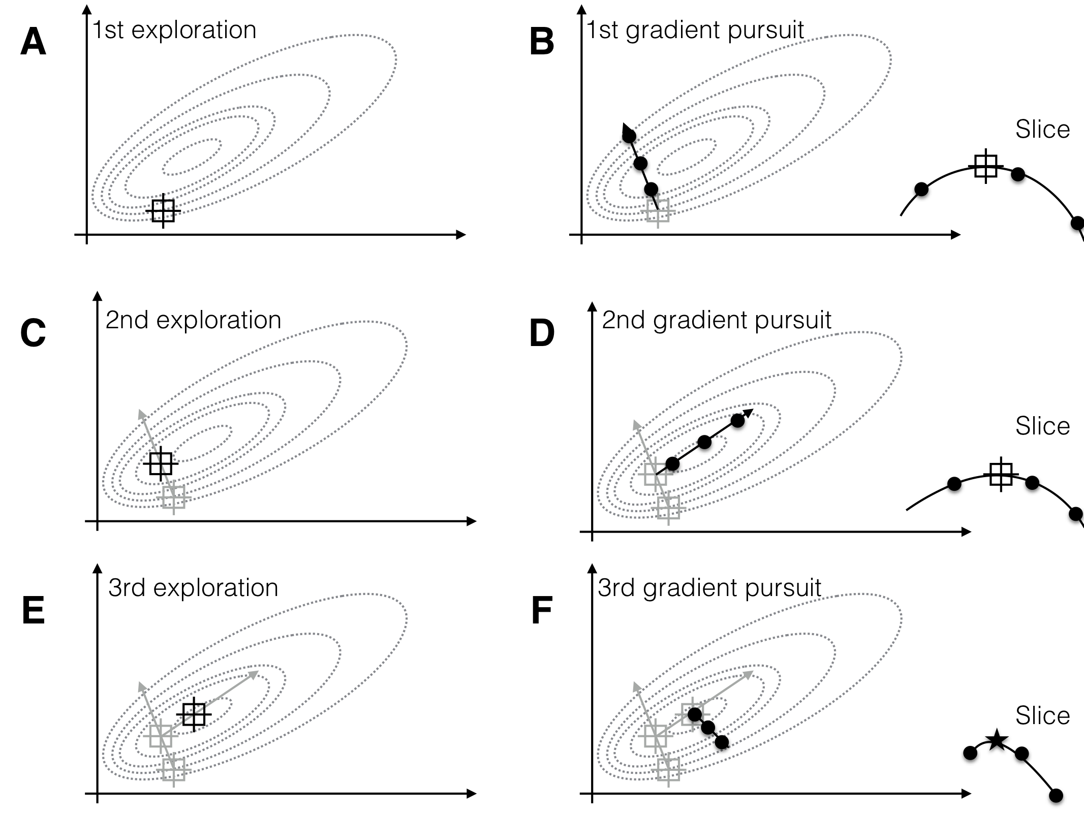
Figure 10.1: Sequential experiments to determine optimum conditions. Three exploration experiments (A,C,E), each followed by a gradient pursuit (B,D,F). Dotted lines: contours of response surface. Black lines and dots: region and points for exploring and gradient pursuit. Inlet curves in panels B,D,F show the slice along the gradient with measured points and resulting maximum.
For implementing this strategy, we need to decide what point to start from; how to approximate the surface \(\phi(\cdot)\) locally; how many and what design points \((x_{1,j},\dots,x_{k,j})\) to choose to estimate this approximation; and how to determine the path of steepest ascent.
Optimizing treatment combinations usually means that we already have a reasonably reliable experimental system, so we use the current experimental condition as our initial point for the optimization. An important aspect here is the reproducibility of the results: if the system or the process under study does not give reproducible results at the starting point, there is little hope that the response surface experiments will give improvements.
The remaining questions are interdependent: we typically choose a simple (polynomial) function to locally approximate the response surface. Our experimental design must then allow the estimation of all parameters of this function, the estimation of the residual variance, and ideally provide information to separate residual variation from lack of fit of the approximation. Determining a gradient is straightforward for a polynomial interpolation function.
We discuss two commonly used models for approximating the response surface: the first-order model requires only a simple experimental design but does not account for curvature of the surface and predicts ever-increasing responses along the path of steepest ascent. The second-order model allows for curvature and has a defined stationary point (a maximum, minimum, or saddle-point), but requires a more complex design for estimating its parameters.
10.3 The First-Order Model
We start our discussion by looking into the first-order model for locally approximating the response surface.
10.3.1 Model
The first-order model for \(k\) quantitative factors (without interactions) is \[ y = f(x_1,\dots,x_k) + e = \beta_0 + \beta_1 x_1 +\cdots+\beta_k x_k +e = \beta_0 + \sum_{i=1}^k \beta_{i} x_i + e\;. \] We estimate its parameters using standard linear regression; the parameter \(\beta_i\) gives the amount by which the expected response increases if we increase the \(i\)th factor from \(x_i\) to \(x_i+1\), keeping all other factors fixed. Without interactions, the predicted change in response is independent of the values of all other factors, and interactions could be added if necessary. We assume a constant error variance \(\text{Var}(e)=\sigma^2\) and justify this by the fact that we explore the response surface only locally.
10.3.2 Path of Steepest Ascent
At any given point \((x_1^*,\dots,x_k^*)\), the gradient of \(f(\cdot)\) is \[ g(x_1^*,\dots,x_k^*) = \left(\beta_1,\dots,\beta_k\right)^T\;, \] and gives the direction with fastest increase in response. This gradient is independent of the factor levels (the function \(g(\cdot)\) does not depend on any \(x_i\)), and the direction of steepest ascent is the same no matter where we start.
In the next iteration, we explore this direction experimentally to find a treatment combination that yields a higher expected response then our starting condition. The local approximation of the true response surface by our first-order model is likely to fail once we venture too far from the starting condition, and we will encounter decreasing responses and increasing discrepancies between the response predicted by the approximation and the response actually measured. One iteration of exploration and gradient pursuit is illustrated in Figure 10.2.
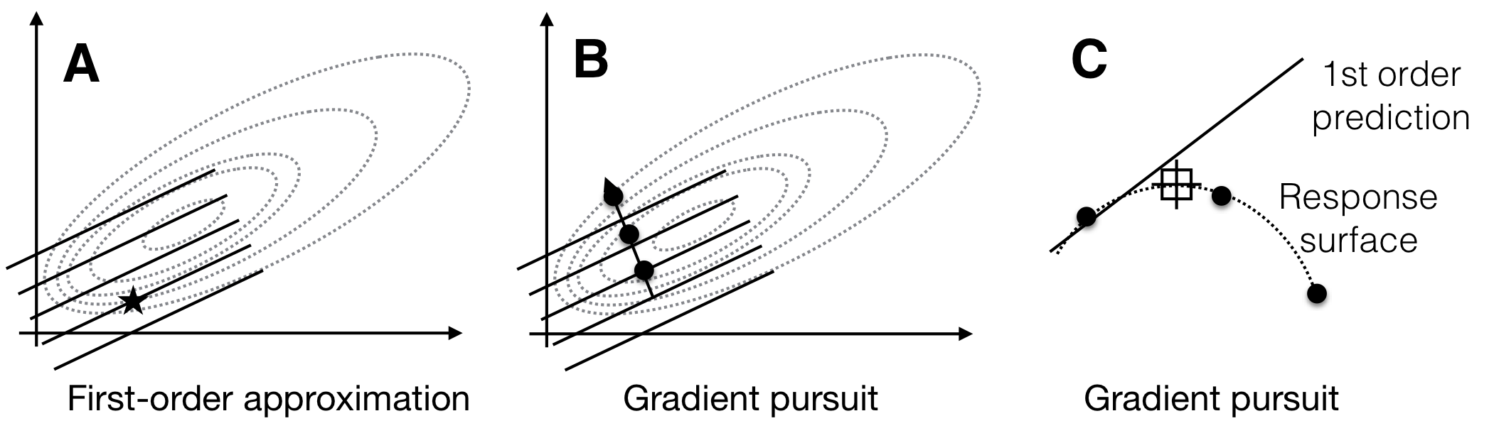
Figure 10.2: Sequential response surface experiment with first-order model. A: The first-order model (solid lines) build around a starting condition (star) approximates the true response surface (dotted lines) only locally. B: The gradient follows the increase of the plane and predicts indefinite increase in response. C: The first-order approximation (solid line) deteriorates from the true surface (dotted line) at larger distances from the starting condition, and the measured responses (points) start to decrease.
10.3.3 Experimental Design
The first-order model with \(k\) factors has \(k+1\) parameters, and estimating these requires at least as many observations at different design points. Two options for an experimental design are shown in Figure 10.3 for a two-factor design.
In both designs, we use several replicates at the starting condition as center points. This allows us to estimate the residual variance independently of any assumed model. Comparing this estimate with the observed discrepancies between any other point of the predicted response surface and its corresponding measured value allows testing the goodness of fit of our model. We also observe each factor at three levels, and can use this information to detect curvature not accounted for by the first-order model.
In the first design (Fig. 10.3A), we keep all factors at their starting condition level, and only change the level for one factor at a time. This yields two axial points for each factor, and the design resembles a coordinate system centered at the starting condition. It requires \(2k+m\) measurements for \(k\) factors and \(m\) center point replicates and is adequate for a first-order model without interactions.
The second design (Fig. 10.3B) is a full \(2^2\)-factorial where all factorial points are considered. This design would allow estimation of interactions between the factors and thus a more complex form of approximation. It requires \(2^k+m\) measurements, but fractional replication reduces the experiment size for larger numbers of factors.
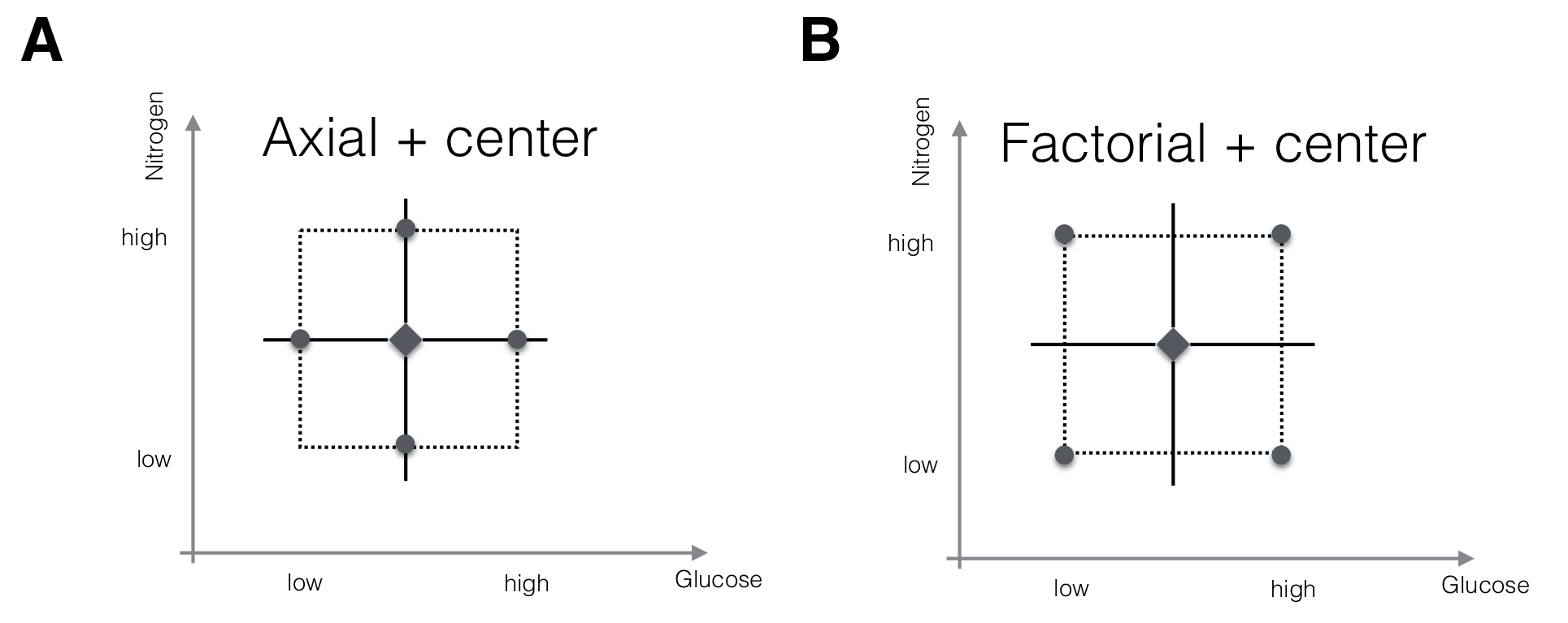
Figure 10.3: Two designs for fitting a first-order RSM with two factors. A: Center points and axial points that modify the level of one factor at a time only allow estimation of main effects, but not of interactions. B: Center points and factorial points increase the experiment size for \(k>2\) but allow estimation of interactions.
A practical problem is the choice for the low and high level of each factor. When chosen too close to the center point, the values for the response will be very similar and it is unlikely that we detect anything but large effects if the residual variance is not very small. When chosen too far apart, we might ‘brush over’ important features of the response surface and end up with a poor approximation. Only subject-matter knowledge can guide us in choosing these levels satisfactorily; for biochemical experiments, one-half and double the starting concentration is often a reasonable first guess.8
10.3.4 Example—Yeast Medium Optimization
For the yeast medium optimization, we consider a \(2^5\)-factorial augmented by six replicates of the center point. This design requires \(2^5+6=38\) runs, which we reduce to \(2^{5-1}+6=22\) runs using a half-replicate of the factorial.
The design is given in Table 10.1, where low and high levels are encoded as \(\pm 1\) and the center level as 0 for each factor, irrespective of the actual amounts or concentrations. The last column shows the measured differences in optical density, with higher values indicating more cells in the corresponding well.
| xGlc | xN1 | xN2 | xVit1 | xVit2 | delta |
|---|---|---|---|---|---|
| Center point replicates | |||||
| 0 | 0 | 0 | 0 | 0 | 81.00 |
| 0 | 0 | 0 | 0 | 0 | 84.08 |
| 0 | 0 | 0 | 0 | 0 | 77.79 |
| 0 | 0 | 0 | 0 | 0 | 82.45 |
| 0 | 0 | 0 | 0 | 0 | 82.33 |
| 0 | 0 | 0 | 0 | 0 | 79.06 |
| Factorial points | |||||
| -1 | -1 | -1 | -1 | 1 | 35.68 |
| 1 | -1 | -1 | -1 | -1 | 67.88 |
| -1 | 1 | -1 | -1 | -1 | 27.08 |
| 1 | 1 | -1 | -1 | 1 | 80.12 |
| -1 | -1 | 1 | -1 | -1 | 143.39 |
| 1 | -1 | 1 | -1 | 1 | 116.30 |
| -1 | 1 | 1 | -1 | 1 | 216.65 |
| 1 | 1 | 1 | -1 | -1 | 47.48 |
| -1 | -1 | -1 | 1 | -1 | 41.35 |
| 1 | -1 | -1 | 1 | 1 | 5.70 |
| -1 | 1 | -1 | 1 | 1 | 84.87 |
| 1 | 1 | -1 | 1 | -1 | 8.93 |
| -1 | -1 | 1 | 1 | 1 | 117.48 |
| 1 | -1 | 1 | 1 | -1 | 104.46 |
| -1 | 1 | 1 | 1 | -1 | 157.82 |
| 1 | 1 | 1 | 1 | 1 | 143.33 |
This encoding yields standardized coordinates with the center point at the origin \((0,0,0,0,0)\) and ensures that all parameters have the same interpretation as one-half the expected difference in response between low and high level, irrespective of the numerical values of the concentrations used in the experiment.
The model allows separation of three sources of variation: (i) the variation explained by the first-order model, (ii) the variation due to lack of fit, and (iii) the pure (sampling and measurement) error. These are quantified by an analysis of variance as shown in Table 10.2.
| Df | Sum Sq | Mean Sq | F value | Pr(>F) | |
|---|---|---|---|---|---|
| FO(Glc, N1, N2, Vit1, Vit2) | 5 | 38102.72 | 7620.54 | 7.94 | 6.30e-04 |
| Residuals | 16 | 15355.32 | 959.71 | ||
| Lack of fit | 11 | 15327.98 | 1393.45 | 254.85 | 3.85e-06 |
| Pure error | 5 | 27.34 | 5.47 |
For the example, the lack of fit is substantial, with a highly significant \(F\)-value, and the first-order approximation is clearly not an adequate description of the response surface. Still, the resulting parameter estimates already give a clear indication for the next round of experimentation along the gradient. Recall that our main goal is to find the direction of highest increase in the response values and we are less interested in finding an accurate description of the surface in the beginning of the experiment.
The pure error is based solely on the six replicates of the center points and consequently has five degrees of freedom. Its variance is about 5.5 and very small compared to the other contributors. This means that the starting point produces highly replicable results and that small differences on the response surface are detectable.
The resulting gradient for this example is shown in Table 10.4, indicating the direction of steepest ascent in standardized coordinates.
| Glc | N1 | N2 | Vit1 | Vit2 |
|---|---|---|---|---|
| -0.32 | 0.17 | 0.89 | -0.09 | 0.26 |
The parameter estimates \(\hat{\beta}_0,\dots,\hat{\beta}_5\) are shown in Table 10.6. The intercept corresponds to the predicted average response at the center point; the empirical average is 81.12, in good agreement with the model.
| Parameter | Estimate | Std. Error | t value | Pr(>|t|) |
|---|---|---|---|---|
| (Intercept) | 85.69 | 6.60 | 12.97 | 6.59e-10 |
| Glc | -15.63 | 7.74 | -2.02 | 6.06e-02 |
| N1 | 8.38 | 7.74 | 1.08 | 2.95e-01 |
| N2 | 43.46 | 7.74 | 5.61 | 3.90e-05 |
| Vit1 | -4.41 | 7.74 | -0.57 | 5.77e-01 |
| Vit2 | 12.61 | 7.74 | 1.63 | 1.23e-01 |
We note that N2 has the largest impact and should be increased, that Vit2 should also be increased, that Glc should be decreased, while N1 and Vit1 seem to have only a comparatively small influence.
10.4 The Second-Order Model
10.4.1 Model
The second-order model adds purely quadratic (PQ) terms \(x_i^2\) and two-way interaction (TWI) terms \(x_i\cdot x_j\) to the first-order model (FO), such that the regression model equation becomes \[ y = f(x_1,\dots,x_k)+ e = \beta_0 + \sum_{i=1}^k \beta_{i} x_i + \sum_{i=1}^k \beta_{ii} x_i^2 + \sum_{i<j}^k \beta_{ij} x_ix_j +e\;, \] and we again assume a constant error variance \(\text{Var}(e)=\sigma^2\) for all points (and can again justify this because we are looking at a local approximation of the response surface). For example, the two-factor second-order response surface approximation is \[ y = \beta_0 + \beta_1\, x_1+\beta_2\, x_2 + \beta_{1,1}\,x_1^2 + \beta_{2,2}\,x_2^2 + \beta_{1,2}\, x_1\,x_2+e\;. \] and only requires estimation of six parameters to describe the true response surface locally. It performs satisfactorily for most problems, at least locally in the vicinity of a given point. Importantly, the model is still linear in the parameters, and parameter estimation can therefore be handled as a standard linear regression problem.
The second-order model allows curvature in all directions and interactions between factors which provides more information about the shape of the response surface. Canonical analysis then allows us to detect ridges along which two or more factors can be varied with only little change to the response and to determine if a stationary point on the surface is a maximum or minimum or a saddle-point where the response increases along one direction, and decreases along another direction. We do not pursue this technique and refer to the references in Section 10.6 for further details.
10.4.2 Path of Steepest Ascent
We find the direction of steepest ascent by calculating the gradient. In contrast to the first-order model the gradient now depends on the position. The path of steepest ascent is then no longer a straight line, but is rather a curved path following the curvature of the response surface.
For example, the first component of the gradient (in direction \(x_1\)) depends on the levels \(x_1,\dots,x_k\) of all treatment factors in the design: \[ (g(x_1,\dots,x_k))_1 = \frac{\partial}{\partial x_1}f(x_1,\dots,x_k)=\beta_1 + 2\beta_{1,1} x_1 + \beta_{1,2} x_2 + \cdots +\beta_{1,k} x_k\;, \] and likewise for the other \(k-1\) components.
10.4.3 Experimental Design
For a second-order model, we need at least three points on each axis to estimate its parameters and we need sufficient combinations of factor levels to estimate the interactions. An elegant way to achieve this is a central composite design (CCD). It combines center points with replication to provide a model-independent estimate of the residual variance, axial points, and a (fractional) factorial design; Figure 10.4 illustrates two designs and their components for a design with three factors.
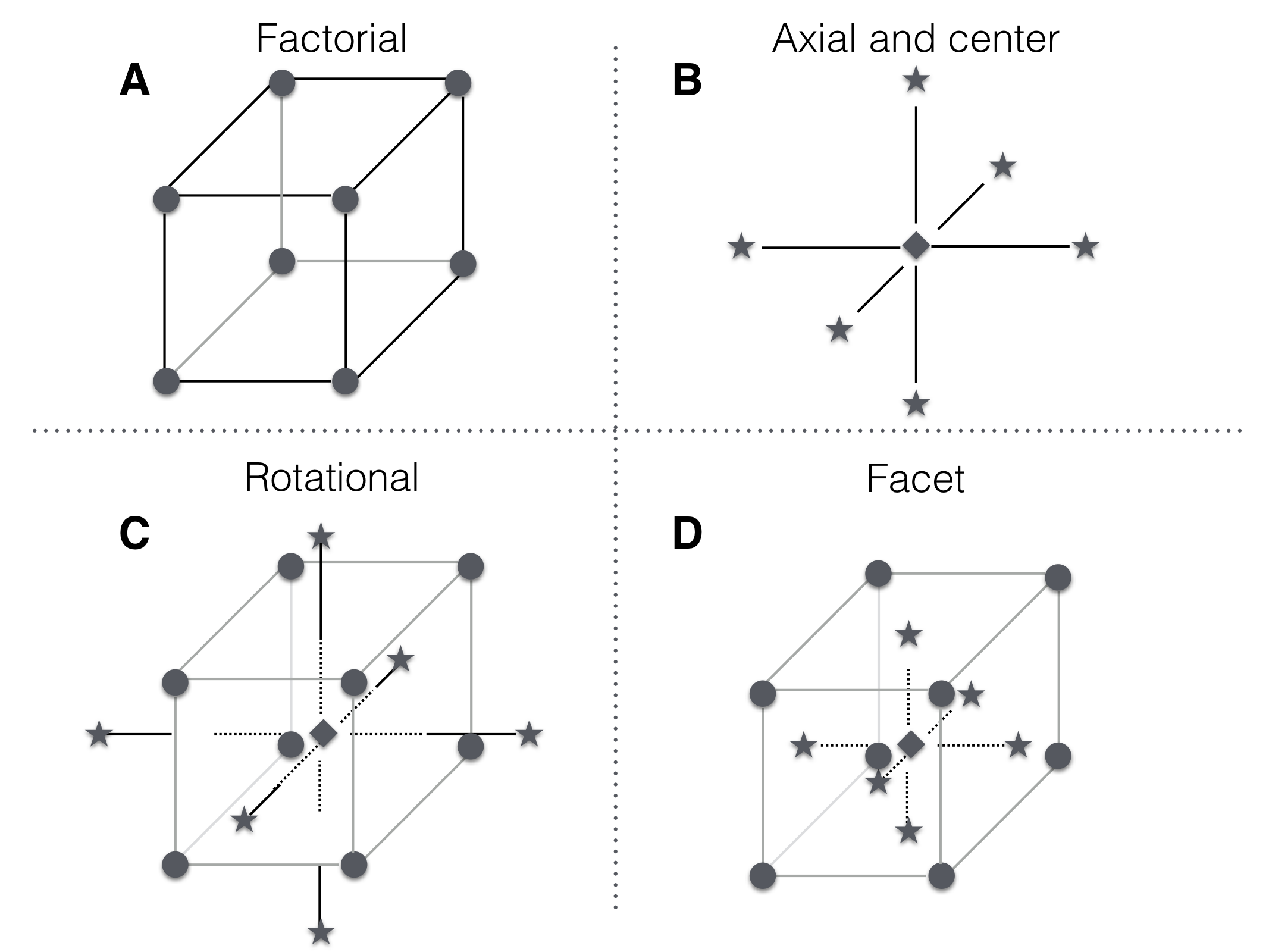
Figure 10.4: A central composite design for three factors. A: Design points for \(2^3\) full factorial. B: Center point location and axial points chosen along axis parallel to coordinate axis and through center point. C: Central composite design with axis points chosen for rotatability. D: Combined design points with axial points chosen on facets introduce no new factor levels.
With \(m\) center point replicates, a central composite design for \(k\) factors requires \(2^k\) factorial points, \(2\cdot k\) axial points, and \(m\) center points. For our example with \(k=5\) factors, the full CCD with six replicates of the center points requires measuring the response for \(32+10+6=48\) settings. The \(2_{\text{V}}^{5-1}\) fractional factorial reduces this number to \(16+10+6=32\) and provides a very economic design.
Choosing Axial Points
In the CCD, we combine axial points and factorial points, and there are two reasonable alternatives for choosing their levels: first, we can choose the axial and factorial points at the same distance from the center point, so they lie on a sphere around the center point (Figure 10.4C). This rotationally symmetric design yields identical standard errors for all parameters and uses levels \(\pm 1\) for factorial and \(\pm\sqrt{k}\) for axial points.
Second, we can choose axial points on the facets of the factorial hyper-cube by using the same low/high levels as the factorial points (Figure 10.4D). This has the advantage that we do not introduce new factor levels, which can simplify the implementation of the experiment. The disadvantage is that the axial points are closer to the center points than are the factorial points and estimates of parameters then have different standard errors, leading to different variances of the model’s predictions depending on the direction.
Blocking a Central Composite Design
The factorial and axial parts of a central composite design are orthogonal to each other. This attractive feature allows a very simple blocking strategy, where we use one block for the factorial points and some of the replicates of the center point, and another block for the axial points and the remaining replicates of the center point. We can then conduct the CCD of our example in two experiments, one with \(16+3=19\) measurements, and the other with \(10+3=13\) measurements, without jeopardizing the proper estimation of parameters. The block size for the factorial part can be further reduced using the techniques for blocking factorials from Section 9.8.
In practice, this property provides considerable flexibility when conducting such an experiment. For example, we might first measure the axial and center points and estimate a first-order model from these data and determine the gradient.
With replicated center points, we are then able to quantify the lack of fit of the model and the curvature of the response surface. We might then decide to continue with the gradient pursuit based on the first-order model if curvature is small, or to conduct a second experiment with factorial and center points to augment the data for estimating a full second-order model.
Alternatively, we might start with the factorial points to determine a model with main effects and two-way interactions. Again, we can continue with these data alone, augment the design with axial points to estimate a second-order model, or augment the data with another fraction of the factorial design to disentangle confounded factors and gain higher precision of parameter estimates.
10.4.4 Sequential Experiments
Next, we measure the response for several experimental conditions along the path of steepest ascent. We then iterate the steps of approximation and gradient pursuit based on the condition with highest measured response along the path.
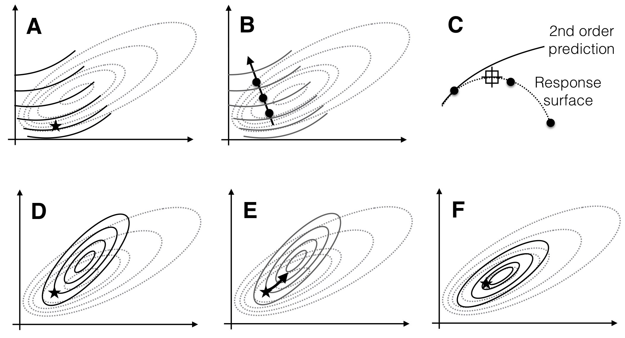
Figure 10.5: Sequential experimentation for optimizing conditions using second-order approximations. A: First approximation (solid lines) of true response surface (dotted lines) around a starting point (star). B: Pursuing the path of steepest ascent yields a new best condition. C: Slice along the path of steepest ascent. D: Second approximation around new best condition. E: Path of steepest ascent based on second approximation. F: Third approximation captures the properties of the response surface around the optimum.
The overall sequential procedure is illustrated in Figure 10.5: the initial second-order approximation (solid lines) of the response surface (dotted lines) is only valid locally (A) and predicts an optimum far from the actual optimum, but pursuit of the steepest ascent increases the response values and moves us closer to the optimum (B). Due to the local character of the approximation, predictions and measurements start to diverge further away from the starting point (C). The exploration around the new best condition predicts an optimum close to the true optimum (D) and following the steepest ascent (E) and a third exploration (F) achieves the desired optimization. The second-order model now has an optimum very close to the true optimum and correctly approximates the factor influences and their interactions locally.
A comparison of predicted and measured responses along the path supplies information about the range of factor levels for which the second-order model provides accurate predictions. A second-order model also allows prediction of the optimal condition directly. This prediction strongly depends on the approximation accuracy of the model and we should treat predicted optima with suspicion if they are far outside the factor levels used for the exploration.
10.5 A Real-Life Example—Yeast Medium Optimization
We revisit our example of yeast medium optimization from Section 9.4. Recall that our goal is to alter the composition of glucose (Glc), monosodium glutamate (nitrogen source N1), a fixed composition of amino acids (nitrogen source N2), and two mixtures of trace elements and vitamins (Vit1 and Vit2) to maximize growth of yeast. Growth is measured as increase in optical density, where higher increase indicates higher cell density. We summarize the four sequential experiments used to arrive at the specification of a new high cell density (HCD) medium (Roberts, Kaltenbach, and Rudolf 2020).
10.5.1 First Response Surface Exploration
Designing the response surface experiments required some consideration to account for the specific characteristics of the experimental setup. There are two factors that most influence the required effort and the likelihood of experimental errors: first, each experiment can be executed on a 48-well plate with cheap ingredients and any experiment size between 1 and 48 requires roughly equivalent effort. That means that we should use a second-order model directly rather than starting with a simpler model and augmenting the data if necessary. We decided to start from a defined yeast medium and use a \(2^{5-1}\) fractional factorial design together with 10 axial points (26 design points without center points) as our first experimental design.
Second, it is very convenient to choose facet axial points, so each medium component has only three instead of five concentrations. We considered sacrificing the rotational symmetry of the design a small price to pay for easier and less error-prone pipetting.
We decided to use six center points to augment the five error degrees of freedom (26 observations in the design for 21 parameters in the second-order model). These allow separating lack of fit from residual variance. By looking at the six resulting growth curves we could also gauge reproducibility of the initial experimental conditions.
We next decided to replicate the fractional factorial part of the CCD in the remaining 16 wells, using a biological replicate with new yeast culture and independent pipetting of the medium compositions. Indeed, the first replicate failed (cf. Section 9.4), and our analysis is based on the second replicate only. Using the remaining 16 wells to complete the \(2^5\)-factorial would have been statistically desirable, but would require more complex pipetting and leave us without any direct replicates except the initial condition.
The resulting increases in optical density (OD) are shown in Figure 10.6. The six values for the center points show excellent agreement, indicating high reproducibility of the experiment. Moreover, the average increase in OD for the starting condition is 81.1, and we already identified a condition with a value of 216.6, corresponding to a 2.7-fold increase.
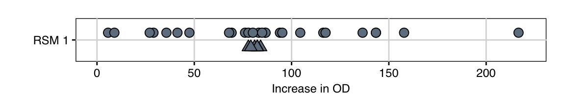
Figure 10.6: Measured increase in OD for first exploration experiment. Triangles indicate center point replicates.
We next estimated the parameters of the second-order approximation based on these observations; the estimates showed several highly significant and large main effects and two-way interactions, while the quadratic terms remained non-significant. This shows that optimization cannot be done iteratively one factor at a time, but that several factors need to be changed simultaneously. The non-significant quadratic terms indicate that either the surface is sufficiently plane around the starting point, or that we chose factor levels too close together or too far apart to detect curvature. The ANOVA table for this model (Table 10.9), however, shows that quadratic terms and two-way interactions as a whole cannot be neglected, but that the first-order part of the model is by far the most important.
| Df | Sum Sq | Mean Sq | F value | Pr(>F) | |
|---|---|---|---|---|---|
| FO(Glc, N1, N2, Vit1, Vit2) | 5 | 43421.11 | 8684.22 | 99.14 | 9.10e-09 |
| TWI(Glc, N1, N2, Vit1, Vit2) | 10 | 15155.26 | 1515.53 | 17.3 | 2.49e-05 |
| PQ(Glc, N1, N2, Vit1, Vit2) | 5 | 289.44 | 57.89 | 0.66 | 6.61e-01 |
| Residuals | 11 | 963.6 | 87.6 | ||
| Lack of fit | 6 | 936.26 | 156.04 | 28.54 | 1.02e-03 |
| Pure error | 5 | 27.34 | 5.47 |
The table also suggests considerable lack of fit, but we expect this at the beginning of the optimization. This becomes very obvious when looking at the predicted stationary point of the approximated surface (Table 10.11), which contains negative concentrations and is far outside the region we explored in the first experiment (note that the units are given in standardized coordinates, so a value of 10 means ten times farther from the center point than our axial points).
| Glc | N1 | N2 | Vit1 | Vit2 |
|---|---|---|---|---|
| 4.77 | 0.38 | -2.37 | 2.19 | 1.27 |
10.5.2 First Path of Steepest Ascent
Based on this second-order model, we calculated the path of steepest ascent for the second experiment in Table 10.12.
| Distance | Glc | N1 | N2 | Vit1 | Vit2 | Predicted | Measured |
|---|---|---|---|---|---|---|---|
| 0.0 | 0.0 | 0.0 | 0.0 | 0.0 | 0.0 | 81.8 | 78.3 |
| 0.5 | -0.2 | 0.1 | 0.4 | 0.0 | 0.1 | 108.0 | 104.2 |
| 1.0 | -0.4 | 0.3 | 0.8 | 0.0 | 0.3 | 138.6 | 141.5 |
| 1.5 | -0.6 | 0.6 | 1.1 | 0.0 | 0.5 | 174.3 | 156.9 |
| 2.0 | -0.8 | 0.8 | 1.4 | 0.1 | 0.8 | 215.8 | 192.8 |
| 2.5 | -1.1 | 1.1 | 1.7 | 0.2 | 1.0 | 263.3 | 238.4 |
| 3.0 | -1.3 | 1.4 | 1.9 | 0.3 | 1.3 | 317.2 | 210.5 |
| 3.5 | -1.5 | 1.7 | 2.1 | 0.4 | 1.5 | 377.4 | 186.5 |
| 4.0 | -1.7 | 2.1 | 2.4 | 0.5 | 1.8 | 444.3 | 144.2 |
| 4.5 | -1.9 | 2.4 | 2.6 | 0.6 | 2.0 | 517.6 | 14.1 |
The first column shows the distance from the center point in standardized coordinates, so this path moves up to 4.5 times further than our axial points. The next columns are the resulting levels for our five treatment factors in standardized coordinates. The column “Predicted” provides the predicted increase in OD based on our second-order approximation.
We experimentally followed this path and took measurements at the indicated medium compositions. This resulted in the measurements given in column “Measured.” We observe a fairly good agreement between prediction and measurement up to about distance 2.5 to 3.0. Thereafter, the predictions keep increasing while measured values drop sharply to almost zero. This is an example of the situation depicted in Figure 10.5C, where the approximation breaks down further from the center point. This is clearly visible when graphing the prediction and measurements in Figure 10.7. Nevertheless, the experimental results show an increase by about 3-fold compared to the starting condition along the path.
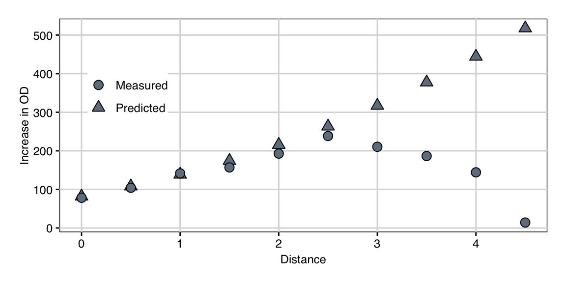
Figure 10.7: Observed growth and predicted values along the path of steepest ascent. Model predictions deteriorate from a distance of about \(2.5-3.0\).
10.5.3 Second Response Surface Exploration
In the next iteration, we explored the response surface locally using a new second-order model centered at the current best condition. We proceeded just as for the first RSM estimation, with a \(2^{5-1}\)-design combined with axial points and six center point replicates.
The 32 observations from this experiment are shown in Figure 10.8 (top row). The new center conditions have consistently higher values than the conditions of the first exploration (bottom row), which is a good indication that the predicted increase is indeed happening in reality. Several conditions show further increase in response, although the fold-changes in growth are considerably smaller than before. The maximal increase from the center point to any condition is about 1.5-fold. This is expected when we assume that we approach the optimum condition.
Figure 10.8: Distribution of measured values for first (bottom) and second (top) exploration experiment with 32 conditions each. Triangles indicate center point replicates.
The center points are more widely dispersed now, which might be due to more difficult pipetting, especially as we originally used a standard medium. The response surface might also show more curvature in the current region, such that deviations from a condition result in larger changes in the response.
Importantly, we do not have to compare the observed values between the two experiments directly, but need only compare a fold-change in each experiment over its center point condition. That means that changes in the measurement scale (which is in arbitrary units) do not affect our conclusions. Here, the observed center point responses of around 230 agree very well with those predicted from the gradient pursuit experiment, so we have confidence that the scales of the two experiments are comparable.
The estimated parameters for a second-order model now present a much cleaner picture: we find only main effects large and significant, and the interaction of glucose with the second nitrogen source (amino acids); all other two-way interactions and the quadratic terms are small. The ANOVA Table 10.14 still indicates some contributions of interactions and purely quadratic terms, but the lack of fit is now negligible. In essence, we are now dealing with a first-order model with one substantial interaction.
| Df | Sum Sq | Mean Sq | F value | Pr(>F) | |
|---|---|---|---|---|---|
| FO(Glc, N1, N2, Vit1, Vit2) | 5 | 89755.57 | 17951.11 | 24.43 | 1.31e-05 |
| TWI(Glc, N1, N2, Vit1, Vit2) | 10 | 33676.72 | 3367.67 | 4.58 | 9.65e-03 |
| PQ(Glc, N1, N2, Vit1, Vit2) | 5 | 28320.87 | 5664.17 | 7.71 | 2.45e-03 |
| Residuals | 11 | 8083.92 | 734.9 | ||
| Lack of fit | 6 | 5977.97 | 996.33 | 2.37 | 1.82e-01 |
| Pure error | 5 | 2105.96 | 421.19 |
The model is still a very local approximation, as is evident from the stationary point far outside the explored region with some values corresponding to negative concentrations (Table 10.16).
| Glc | N1 | N2 | Vit1 | Vit2 |
|---|---|---|---|---|
| 1.02 | -6.94 | 1.25 | -11.76 | -2.54 |
10.5.4 Second Path of Steepest Ascent
Based on this second model, we again calculated the path of steepest ascent and followed it experimentally. The predictions and observed values in Figure 10.9 show excellent agreement, even though the observed values are consistently higher. The systematic shift already occurs for the starting condition and a likely explanation is the gap of several months between second exploration experiment and the gradient pursuit experiment, leading to differently calibrated measurement scales.
This systematic shift is not a problem in practice, since we have the same center point condition as a baseline measurement, and in addition are interested in changes in the response along the path, and less in their actual values. Along the path, the response is monotonically increasing, resulting in a further 2.2-fold increase compared to our previous optimum at the last condition.
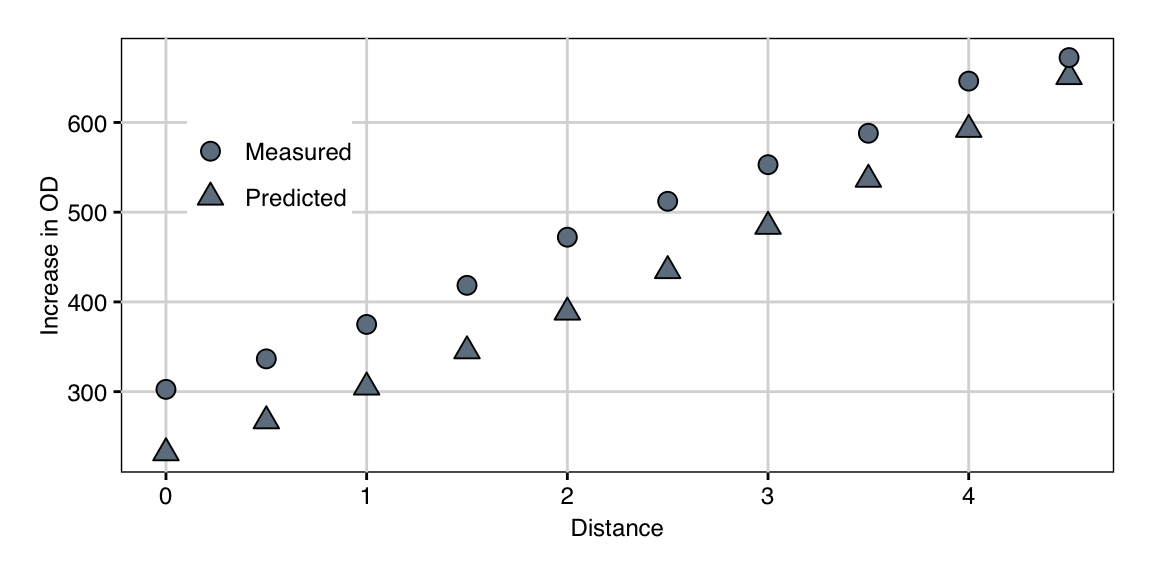
Figure 10.9: Observed growth and predicted values along the second path of steepest ascent.
Although our model predicts that further increase in growth is possible along the gradient, we stopped the experiment at this point. The wells of the 48-well plate were now crowded with cells and several components were so highly concentrated that salts started to fall out from the solution at the distance-5.0 medium composition.
10.5.5 Conclusion
Overall, we achieved a 3-fold increase in the first iteration, followed by another increase of 2.2-fold in the second iteration, yielding an overall increase in growth of about 6.8-fold. Given that previous manual optimization resulted in a less than 3-fold increase overall, this highlights the power of experimental design and systematic optimization of the medium composition.
We summarize the data of all four experiments in Figure 10.10. The vertical axis shows the four sequential experiments and the horizontal axis the increase in OD for each tested condition. Round points indicate trial conditions of the experimental design for RSM exploration or gradient pursuit, with grey shading denoting two independent replicates. During the second iteration, additional standard media (YPD and SD) were also measured to provide a direct comparison against established alternatives. The second gradient pursuit experiment repeated previous exploration points for direct comparison.

Figure 10.10: Summary of data acquired during four experiments in sequential response surface optimization. Additional conditions were tested during second exploration and gradient pursuit (point shape), and two replicates were measured for both gradients (point shading). Initial starting medium is shown in black.
We noted that while increase in OD was excellent, the growth rate was much slower compared to the starting medium composition. We addressed this problem by changing our optimality criterion from the simple increase in OD to an increase penalized by duration. Using the data from the second response surface approximation, we calculated a new path of steepest ascent based on this modified criterion and arrived at the final high-cell density medium which provides the same increase in growth with rates comparable to the initial medium (Roberts, Kaltenbach, and Rudolf 2020).
10.6 Notes and Summary
Notes
Sequential experimentation for optimizing a response was already discussed in Hotelling (1941), and the response surface methodology was introduced and popularized for engineering statistics by George Box and co-workers (Box and Wilson 1951; Box and Hunter 1957; Box 1954); a current review is Khuri and Mukhopadhyay (2010). Two relevant textbooks are the introductory account in Box, Hunter, and Hunter (2005) and the more specialized text by Box and Draper (2007); both also discuss canonical analysis. The classic Cochran and Cox (1957) also provides a good overview. The use of RSM in the context of biostatistics is reviewed in Mead and Pike (1975).
Using R
The rsm package (Lenth 2009) provides the function rsm() to estimate response surface models; they are specified using R’s formula framework extended by convenience functions (Table 10.17). Coding of data into \(-1/0/+1\) coordinates is done using coded.data(), and steepest() predicts the path of steepest ascent. Central composite designs (with blocking) are generated by the ccd() function.
| Shortcut | Meaning | Example for two factors |
|---|---|---|
FO() |
First-order | \(\beta_0+\beta_1\, x_1+\beta_2\, x_2\) |
PQ() |
Pure quadratic | \(\beta_{1,1}\, x_1^2 + \beta_{2,2}\, x_2^2\) |
TWI() |
Two-way interactions | \(\beta_{1,2}\, x_1\,x_2\) |
SO() |
Second-order | \(\beta_0+\beta_1\, x_1+\beta_2\, x_2+\beta_{1,2}\, x_1\,x_2+\beta_{1,1}\, x_1^2 + \beta_{2,2}\, x_2^2\) |
Summary
Response surface methods provide a principled way for finding optimal experimental conditions that maximize (or minimize) the measured response. The main idea is to create an experimental design for estimating a local approximation of the response surface around a given point, determine the path of steepest ascent using the approximation model and then experimentally explore this path. If a ‘better’ experimental condition is found, the process is repeated from this point until a satisfactory condition is found.
A commonly used design for estimating the approximation model is the central composite design. It consists of a (fractional) factorial design augmented by axial points. Conveniently, axial points and the factorial points are orthogonal and this allows us to implement the design in several stages, where individual smaller experiments are run for the axial points and for (parts of the fractional) factorial points. Multiple replicates of the center point allow separation of lack of fit of the model from residual variance.
This requires that we use a log-scale for the levels of the treatment factors.↩︎