Chapter 9 Many Treatment Factors: Fractional Factorial Designs
9.1 Introduction
Factorial treatment designs are necessary for estimating factor interactions and offer additional advantages (Chapter 6). However, their implementation is challenging if we consider many factors or factors with many levels, because the number of treatments might then require prohibitive experiment sizes. Large factorial experiments also pose problems for blocking, if reasonable block sizes that ensure homogeneity of the experimental material within a block are smaller than the number of treatment level combinations.
For example, a factorial treatment structure with five factors of two levels each has \(2^5=32\) treatment combinations. An experiment with 32 experimental units then has no residual degrees of freedom, but two full replicates of this design already require 64 experimental units. If each factor has three levels, the number of treatment combinations increases drastically to \(3^5=243\).
On the other hand, we might justify the assumption of effect sparsity: high-order interactions are often negligible, especially if interactions of lower orders already have small effect sizes. The key observation for reducing the experiment size is that a large portion of model parameters relate to higher-order interactions: in a \(2^5\)-factorial, there are 32 model parameters: one grand mean, five main effects, ten two-way interactions, ten three-way interactions, five four-way interactions, and one five-way interaction. The number of higher-order interactions and their parameters grows fast with increasing number of factors as shown in Table 9.1 for factorials with two factor levels and 3 to 7 factors.
If we ignore three-way and higher interactions in the example, we remove 16 parameters from the model equation and only require 16 observations for estimating the remaining model parameters; this is known as a half-fraction of the \(2^5\)-factorial. Of course, the ignored interactions do not simply vanish, but their effects are now confounded with those of lower-order interactions or main effects. The question then arises: which 16 out of the 32 possible treatment combinations should we consider such that no effect of interest is confounded with a non-negligible effect?
| Factorial | 0 | 1 | 2 | 3 | 4 | 5 | 6 | 7 |
|---|---|---|---|---|---|---|---|---|
| k=3 | 1 | 3 | 3 | 1 | ||||
| k=4 | 1 | 4 | 6 | 4 | 1 | |||
| k=5 | 1 | 5 | 10 | 10 | 5 | 1 | ||
| k=6 | 1 | 6 | 15 | 20 | 15 | 6 | 1 | |
| k=7 | 1 | 7 | 21 | 35 | 35 | 21 | 7 | 1 |
In this chapter, we discuss the construction and analysis of fractional replications of \(2^k\)-factorial designs where all \(k\) treatment factors have two levels. This restriction is often sufficient for practical experiments with many factors, where interest focuses on identifying relevant factors and low-order interactions. We first consider generic factors which we call A, B and so forth, and denote their two levels generically as low (or \(-1\)) and high (or \(+1\)).
We also extend the idea of fractional replication to deliberately confound some effects with blocks. This allows us to implement a \(2^5\)-factorial in blocks of size 16, for example. By altering the confounding between pairs of blocks, we can still recover all effects, albeit with reduced precision.
9.2 Aliasing in the \(2^3\)-Factorial
9.2.1 Introduction
We begin our discussion with the simple example of a \(2^3\)-factorial treatment structure in a completely randomized design. We denote the treatment factors as A, B, and C and their levels as \(A\), \(B\), and \(C\) with values \(-1\) and \(+1\), generically called the low and high level, respectively. Recall that main effects and interactions (of any order) all have one degree of freedom in a \(2^k\)-factorial; hence, we can encode the two independent levels of an interaction as \(-1\) and \(+1\). We define the level by multiplying the levels of the constituent factors: for \(A=-1\), \(B=+1\), \(C=-1\), the level of A:B is \(AB=A\cdot B=-1\) and the level of A:B:C is \(ABC=A\cdot B\cdot C=+1\).
It is also convenient to use an additional shorthand notation for a treatment combination, where we use a character string containing the lower-case letter of a treatment factor if it is present on its high level, and no letter if it is present on its low level. For example, we write \(abc\) if A, B, C are on level \(+1\), and all potential other factors are on the low level \(-1\), and \(ac\) if A and C are on the high level, and B on its low level. We denote a treatment combination with all factors on their low level by \((1)\). For a \(2^3\)-factorial, the eight different treatments are then \((1)\), \(a\), \(b\), \(c\), \(ab\), \(ac\), \(bc\), and \(abc\).
For example, testing compositions for growth media with factors Carbon with levels Glc (glucose) and Fru (fructose), Nitrogen with levels low and high, and Vitamin with levels Mix 1 and Mix 2 leads to a \(2^3\)-factorial with the 8 possible treatment combinations shown in Table 9.2.
| Carbon | Nitrogen | Vitamin | A | B | C | AB | AC | BC | ABC | Shorthand |
|---|---|---|---|---|---|---|---|---|---|---|
Glc |
low |
Mix 1 |
\(-1\) | \(-1\) | \(-1\) | \(+1\) | \(+1\) | \(+1\) | \(-1\) | \((1)\) |
Glc |
low |
Mix 2 |
\(-1\) | \(-1\) | \(+1\) | \(+1\) | \(-1\) | \(-1\) | \(+1\) | \(c\) |
Glc |
high |
Mix 1 |
\(-1\) | \(+1\) | \(-1\) | \(-1\) | \(+1\) | \(-1\) | \(+1\) | \(b\) |
Glc |
high |
Mix 2 |
\(-1\) | \(+1\) | \(+1\) | \(-1\) | \(-1\) | \(+1\) | \(-1\) | \(bc\) |
Fru |
low |
Mix 1 |
\(+1\) | \(-1\) | \(-1\) | \(-1\) | \(-1\) | \(+1\) | \(+1\) | \(a\) |
Fru |
low |
Mix 2 |
\(+1\) | \(-1\) | \(+1\) | \(-1\) | \(+1\) | \(-1\) | \(-1\) | \(ac\) |
Fru |
high |
Mix 1 |
\(+1\) | \(+1\) | \(-1\) | \(+1\) | \(-1\) | \(-1\) | \(-1\) | \(ab\) |
Fru |
high |
Mix 2 |
\(+1\) | \(+1\) | \(+1\) | \(+1\) | \(+1\) | \(+1\) | \(+1\) | \(abc\) |
9.2.2 Effect Estimates
In a \(2^k\)-factorial, we estimate main effects and interactions as simple contrasts by subtracting the sum of responses of all observations with the corresponding factors on the ‘low’ level \(-1\) from those with the factors on the ‘high’ level \(+1\). For our example, we estimate the main effect of Carbon (or generically A) by subtracting from each observation with fructose (‘high’) the corresponding observation with glucose (‘low’) with nitrogen and vitamin on the same level, and averaging: \[ \text{A main effect} = \frac{1}{4}\left(\,(a-(1)) + (ab-b) + (ac-c) + (abc-bc)\,\right)\;. \] This is equivalent to calculating the Carbon main effect by averaging the difference between the sum of observations with glucose (‘low’) and the sum of observations with fructose (‘high’). In terms of Table 9.2, this amounts to adding all those observations for which \(A=+1\), namely \(a, ab, ac, abc\) and subtracting the sum of all observations for which \(A=-1\), namely \((1), b, c, bc\). This yields \[ \text{A main effect} = \frac{1}{4}\left(\underbrace{(a+ab+ac+abc)}_{A=+1}-\underbrace{((1)+b+c+bc)}_{A=-1}\right)\;, \] which we see is simply the previous calculation with terms grouped differently.
A two-way interaction is a difference of differences and we find the interaction of B with C by first finding the difference between them for A on the low level and for A on the high level: \[ \frac{1}{2}\underbrace{\left((abc-ab)\,-\,(ac-a)\right)}_{\text{if }A=+1} \quad\text{and}\quad \frac{1}{2}\underbrace{\left((bc-b)\,-\,(c-(1))\right)}_{\text{if }A=-1}\;. \] The interaction effect is then the average of these two estimates \[\begin{align*} \text{B:C interaction} &= \frac{1}{2} \left(\;\frac{1}{2}\Big((abc-ab)-(ac-a)\Big)+\frac{1}{2}\Big((bc-b)-(c-(1))\Big)\;\right) \\ &= \frac{1}{4} \left(\; \underbrace{(abc+bc+a+(1))}_{BC=+1}\,-\,\underbrace{(ab+ac+b+c)}_{BC=-1}\; \right)\;. \end{align*}\] This value is equivalently found by taking the difference between observations with \(BC=+1\) (the interaction at its ‘high’ level) and \(BC=-1\) (the interaction at its ‘low’ level) and averaging. The other interaction effects are estimated by contrasting the corresponding observations for \(AB=\pm 1\), \(AC=\pm 1\), and \(ABC=\pm 1\), respectively.
9.2.3 Reduction to Four Treatment Combinations
We are interested in reducing the size of the experiment and for reasons that will become clear shortly, we choose a design based on measuring the response for four out of the eight treatment combinations. This will only allow estimation of four parameters in the linear model, and exactly which parameters can be estimated depends on the treatments chosen. The question then is: which four treatment combinations should we select?
We investigate three specific choices to get a better understanding of the consequences for effect estimation. The designs are illustrated in Figure 9.1, where treatment level combinations form a cube with eight vertices, from which four are selected in each case.
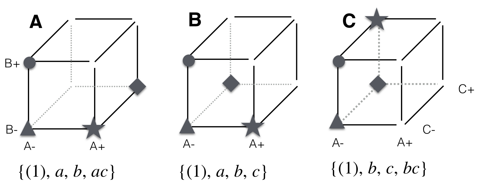
Figure 9.1: Subsets of a \(2^3\)-factorial. A: Arbitrary choice of treatment combinations leads to problems in estimating any effects properly. B: One variable at a time (OVAT) design. C: Keeping one factor at a constant level confounds this factor with the grand mean and creates a \(2^2\)-factorial of the remaining factors.
First, we arbitrarily select the four treatment combinations \((1), a, b, ac\) (Fig. 9.1A). With this choice, none of the main effects or interaction effects can be estimated using all four observations. For example, an estimate of the A main effect involves \(a-(1)\), \(ab-b\), \(ac-c\), and \(abc-bc\), but only \(a-(1)\) is available in this experiment. Compared to a factorial experiment in four runs, this choice of treatment combinations thus allows using only one-half of the available data for estimating this effect. If we follow the above logic and contrast the observations with A at the high level with those with A at the low level, thereby using all data, then the main effect is estimated as \((ac+a)-(b+(1))\) and leads to a biased and incorrect estimate of the main effect, since the other factors are at ‘incompatible’ levels. Similar problems arise for B and C main effects, where only \(b-(1)\), respectively \(ac-a\) are available. None of the interactions can be estimated from these data and we are left with a very unsatisfactory muddle of biased estimates.
Next, we try to be more systematic and select the four treatment combinations \((1), a, b, c\) (Fig. 9.1B) where all factors occur on low and high levels. Again, main effect estimates are based on half of the data for each factor, but their calculation is now simpler: \(a-(1)\), \(b-(1)\), and \(c-(1)\), respectively. Each estimate involves the same level \((1)\) and only two of four observations are used. This design resembles a one variable at a time experiment, where effects can be estimated individually for each factor, but no estimates of interactions are available. All advantages of a factorial treatment design are then lost.
Finally, we select the four treatment combinations \((1), b, c, bc\) with A on the low level (Fig. 9.1C). This design is effectively a \(2^2\)-factorial with treatment factors B and C and allows estimation of their main effects and their interaction, but no information is available on any effects involving the treatment factor A. For example, we estimate the B main effect as \((bc+b)\,-\,(c+(1))\) using all data, and the B:C interaction as \((bc-b)-(c-(1))\). If we look more closely into Table 9.2, we find a simple confounding structure: the level of B is always the negative of A:B. In other words, the two effects are completely confounded in this design, and \((bc+b)\,-\,(c+(1))\) is in fact an estimate of the difference of the B main effect and the A:B interaction. Similarly, C is the negative of A:C, and B:C is the negative of A:B:C. Finally, the grand mean is confounded with the A main effect; this makes sense since any estimate of the overall average is based only on the ‘low’ level of A.
9.2.4 The Half-Replicate or Fractional Factorial
Neither of the previous three choices provided a convincing reduction of the factorial design. We now discuss a fourth possibility, the half-replicate of the \(2^3\)-factorial, called a \(2^{3-1}\)-fractional factorial. The main idea is to deliberately alias a high-order interaction with the grand mean. For a \(2^3\)-factorial, we alias the three-way interaction A:B:C by selecting either those four treatment combinations that have \(ABC=-1\) or those that have \(ABC=+1\). We call the corresponding equation the generator of the fractional factorial; the two possible sets are shown in Figure 9.2. With either choice, we find three more effect aliases by consulting Table 9.2. For example, using \(ABC=+1\) as our generator yields the four treatment combinations \(a, b, c, abc\) and we find that A is completely confounded with B:C, B with A:C, and C with A:B.
In this design, any estimate thus corresponds to the sum of two effects. For example, \((a+abc)-(b+c)\) estimates the sum of A and B:C: first, the main effect of A is found as the difference of the runs \(a\) and \(abc\) with A on its high level, and the runs \(b\) and \(c\) with A on its low level: \((a+abc)-(b+c)\). Second, we contrast runs with B:C on the high level (\(a\) and \(abc\)) with those with B:C on its low level (\(b\) and \(c\)) for estimating the B:C interaction effect, which is again \((a+abc)-(b+c)\).
The fractional factorial based on this generator hence deliberately aliases each main effect with a two-way interaction, and the grand mean with the three-way interaction. Each estimate is then the sum of the two aliased effects. Moreover, we note that by pooling the treatment combinations over levels of one of the three factors, we create three different \(2^2\)-factorials for the two remaining factors as seen in Figure 9.2. For example, ignoring the level of C leads to the full factorial in A and B. This is a consequence of the aliasing, as C is completely confounded with A:B.
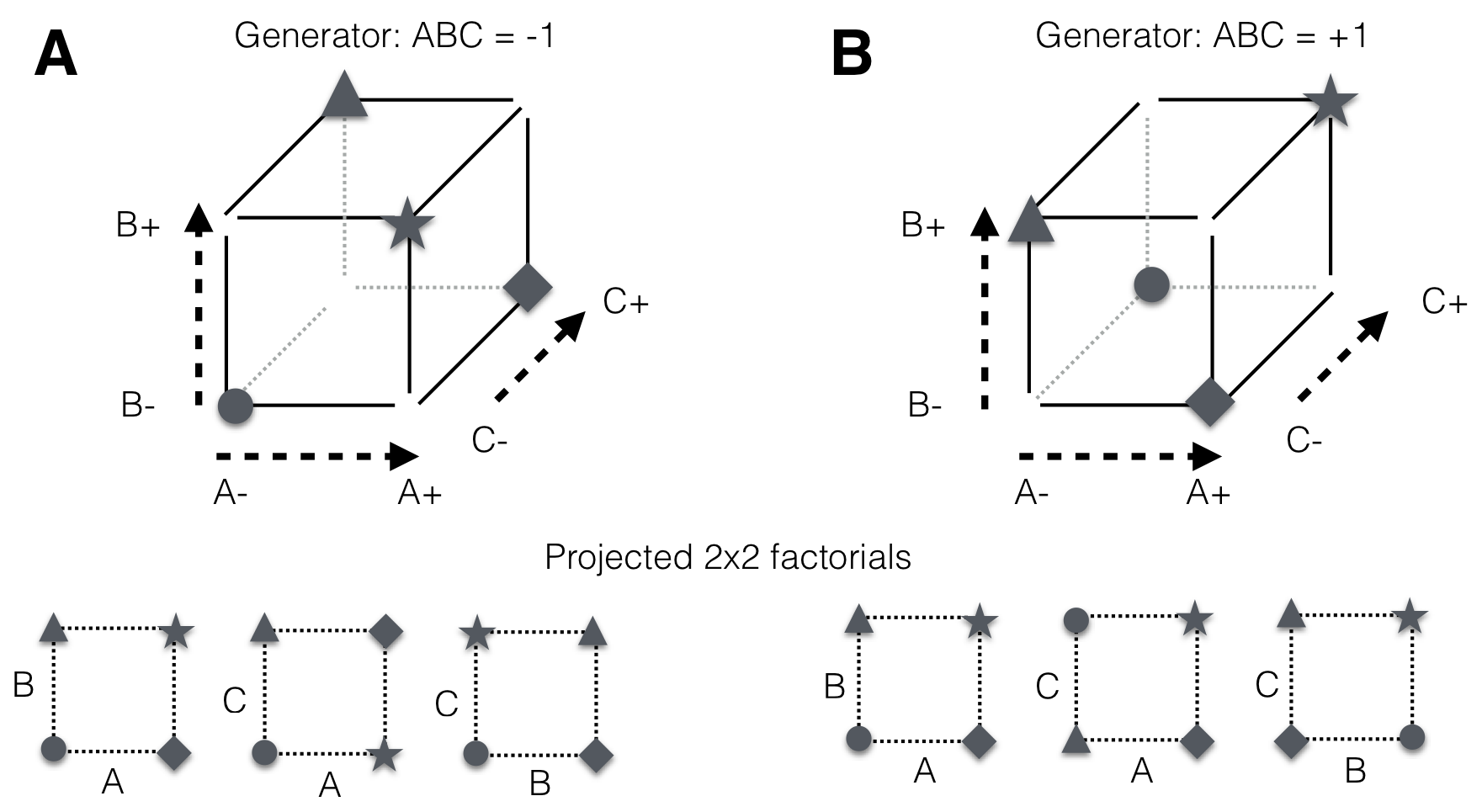
Figure 9.2: The two half-replicates of a \(2^3\)-factorial with three-way interaction and grand mean confounded. Any projection of the design to two factors yields a full \(2^2\)-factorial design and main effects are confounded with two-way interactions. A: Design based on low level of three-way interaction; B: Complementary design based on high level.
The confounding of different effects can be described by the alias sets, where each set contains the effects that cannot be distinguished. For the generator \(ABC=+1\), the alias sets are \[ \{1, ABC\}, \quad \{A, BC\}, \quad \{B, AC\}, \quad \{C, AB\}\;, \] and for the generator \(ABC=-1\), the alias sets are \[ \{1, -ABC\}, \quad \{A, -BC\}, \quad \{B, -AC\}, \quad \{C, -AB\}\;. \] Estimation of the A main effect, for example, is only possible if the B:C interaction is zero in line with our previous observations. A more detailed discussion of confounding in terms of the parameters of the underlying linear model is given in Section 9.9.
9.3 Aliasing in the \(2^k\)-Factorial
The half-replicate of a \(2^3\)-factorial still does not provide an entirely convincing example for the usefulness of fractional factorial designs due to the complete confounding of main effects and two-way interactions, both of which are typically of great interest. With more factors in the treatment structure, however, we are able to alias interactions of higher order and confound low-order interactions of interest with high-order interactions that we might assume negligible.
9.3.1 Using Generators
The generator or generating equation provides a convenient way for constructing fractional factorial designs. The generator is a word written by concatenating the factor letters, such that \(AB\) denotes a two-way interaction, and our previous example \(ABC\) is a three-way interaction; the special ‘word’ \(1\) denotes the grand mean. A generator is then a formal equation that identifies two words and enforces the equality of the corresponding treatment combinations. In our \(2^{3-1}\) design, the generator \[ ABC=+1 \] selects all those rows in Table 9.2 for which the relation is true and A:B:C is on the high level.
A generator determines the effect confounding of the experiment: the generator itself is one confounding and \(ABC=+1\) describes the complete confounding of the the three-way interaction A:B:C with the grand mean.
From the generator, we can derive all other confoundings by simple algebraic manipulation. By formally ‘multiplying’ the generator with an arbitrary word, we find a new relation between effects. In this manipulation, the multiplication with the letter \(+1\) leaves the equation unaltered, multiplication with \(-1\) inverses signs, and a product of two identical letters yields \(+1\). For example, multiplying our generator \(ABC=+1\) with the word \(B\) yields \[ ABC\cdot B=(+1)\cdot B \iff AC=B\;. \] In other words, the B main effect is confounded with the A:C interaction. Similarly, we find \(AB=C\) and \(BC=A\) as two further confounding relations by multiplying the generator with \(C\) and \(A\), respectively.
Further trials with manipulating the generator show that we can obtain no additional relations. For example, multiplying \(ABC=+1\) with the word \(AB\) yields \(C=AB\) again, and multiplying this relation with \(C\) yields \(C\cdot C=AB\cdot C\iff +1=ABC\), the original generator. This means that indeed, we have fully confounded four pairs of effects and no others. In general, a generator for a \(2^k\)-factorial produces \(2^k/2=2^{k-1}\) alias relations between factors, so we have a direct way to check if we found all. In our example, \(2^3/2=4\), so our relations \(ABC=+1\), \(AB=C\), \(AC=B\), and \(BC=A\) cover all existing aliases.
This property also means that we arrive at exactly the same set of alias relations, no matter which of them we choose as our generator. For example, instead of \(ABC=+1\), we might choose \(A=BC\); this selects the same set of rows and implies the same set of confounding relations. Usually, we use a generator that aliases the highest-order interaction with the grand mean and yields the least severe confounding.
Generators provide a systematic way for aliasing that results in interpretable effect estimates with known confoundings. A generator selects one-half of the possible treatment combinations and this is the reason why we set out to choose four rows in our first example.
We briefly note that our first and second choices in Section 9.2.3 are not based on a generator, leaving us with a complex partial confounding of effects. In contrast, our third choice selected all treatments with A on the low level and does have a generator, namely \[ A=-1\;. \] Algebraic manipulation then shows that this design implies the additional three alias relations \(AB=-B\), \(AC=-C\), and \(ABC=-BC\). In other words, any effect involving the factor A is confounded with another effect not involving that factor, which we easily verify from Table 9.2.
9.3.2 Half-Replicates
Generators and their algebraic manipulation provide an efficient way for finding the confoundings in higher-order factorials, where looking at the corresponding table of treatment combinations quickly becomes unfeasible. As we can see from the algebra, the most useful generator is always confounding the grand mean with the highest-order interaction.
For four factors, this generator is \(ABCD=+1\) and we expect that there are \(2^4/2=8\) relations in total. Multiplying with any letter reveals that main effects are then confounded with three-way interactions, such as \(ABCD=+1\iff BCD=A\) after multiplying with \(A\), and similarly \(B=ACD\), \(C=ABD\), and \(D=ABC\). Moreover, by multiplication with two-letter words we find that all two-way interactions are confounded with other two-way interactions, namely via the three relations \(AB=CD\), \(AC=BD\), and \(AD=BC\). We thus found eight relations and can be sure that there are no others.
The resulting confounding is already an improvement over fractions of the \(2^3\)-factorial, especially if we can make the argument that three-way interactions can be neglected and we thus have direct estimates of all main effects. If we find a significant and large two-way interaction—A:B, say—then we cannot distinguish if it is A:B, its alias C:D, or a combination of the two that produces the effect. Subject-matter considerations might be available to separate these possibilities. If not, there is at least a clear goal for a subsequent experiment to disentangle the two interaction effects.
Things improve further for five factors and the generator \(ABCDE=+1\) which reduces the number of treatment combinations from \(2^5=32\) to \(2^{5-1}=16\). Now, main effects are confounded with four-way interactions, and two-way interactions are confounded with three-way interactions. Invoking the principle of effect sparsity and neglecting the three- and four-way interactions yields main effects and two-way interactions as the estimated parameters.
Main effects and two-way interactions are confounded with interactions of order four or higher for factorials with six factors and more, and we can often assume that these interactions are negligible.
9.4 A Real-Life Example—Yeast Medium Composition
As a concrete example of a fractional factorial treatment design, we discuss an experiment conducted during the sequential optimization of a yeast growth medium, which we discuss in more detail in Chapter 10. For now, we concentrate on determining the individual and combined effects of five medium ingredients—glucose Glc, two different nitrogen sources N1 (monosodium glutamate) and N2 (an amino acid mixture), and two vitamin sources Vit1 and Vit2—on the resulting number of yeast cells. Different combinations of concentrations of these ingredients are tested on a 48-well plate, and the growth curve is recorded for each well by measuring the optical density over time. We use the increase in optical density (\(\Delta\text{OD}\)) between onset of growth and flattening of the growth curve at the diauxic shift as a rough but sufficient approximation for increase in number of cells.
9.4.1 Experimental Design
To determine how the five medium components influence the growth of the yeast culture, we use the composition of a standard medium as a reference point, and simultaneously alter the concentrations of the five components. For this, we select two concentrations per component, one lower, the other higher than the standard, and consider these as two levels for each of five treatment factors. The treatment structure is then a \(2^5\)-factorial and would in principle allow estimation of the main effects and all two-, three-, four-, and five-factor interactions when we use all \(32\) possible combinations. However, a single replicate requires two-thirds of a 48-well plate and this is undesirable because we would like sufficient replication and also be able to compare several yeast strains in the same plate. Both requirements can be accommodated by using a half-replicate of the \(2^5\)-factorial with 16 treatment combinations, such that three independent experiments fit on a single plate.
A generator \(ABCDE=+1\) confounds the main effects with four-way interactions, which we consider negligible for this experiment. Still, two-way interactions are confounded with three-way interactions, and in the first implementation we assume that three-way interactions are much smaller than two-way interactions. We can then interpret main effect estimates directly, and assume that estimates of parameters involving two-way interactions have only small contributions from the corresponding three-way interactions. The design is shown in Table 9.3.
| Glucose | Nitrogen 1 | Nitrogen 2 | Vitamin 1 | Vitamin 2 | OD 1 | OD 2 | |||||||||||||||||||||||||||||||||||||||||||||||||||||||||||||||||||||||||||||||||||||||||||||||||||||||||||||||||||||||||||||||||||||||||||||||||||||||||||||||||||||||||||||||||||||||||||||||||||||||||||||||||||||||||||||||||||||||||||||||||||||||||||||||||||||||||||||||||||||||||||||||||||||||||||||||||||||||||||||||||||||||||||||||||||||||||||||||||||||||||||||||||||||||||||||||||||||||||||||||||||||||||||||||||||||||||||||||||||||||||||||||||||||||||||||||||||||||||||||||||||||||||
|---|---|---|---|---|---|---|---|---|---|---|---|---|---|---|---|---|---|---|---|---|---|---|---|---|---|---|---|---|---|---|---|---|---|---|---|---|---|---|---|---|---|---|---|---|---|---|---|---|---|---|---|---|---|---|---|---|---|---|---|---|---|---|---|---|---|---|---|---|---|---|---|---|---|---|---|---|---|---|---|---|---|---|---|---|---|---|---|---|---|---|---|---|---|---|---|---|---|---|---|---|---|---|---|---|---|---|---|---|---|---|---|---|---|---|---|---|---|---|---|---|---|---|---|---|---|---|---|---|---|---|---|---|---|---|---|---|---|---|---|---|---|---|---|---|---|---|---|---|---|---|---|---|---|---|---|---|---|---|---|---|---|---|---|---|---|---|---|---|---|---|---|---|---|---|---|---|---|---|---|---|---|---|---|---|---|---|---|---|---|---|---|---|---|---|---|---|---|---|---|---|---|---|---|---|---|---|---|---|---|---|---|---|---|---|---|---|---|---|---|---|---|---|---|---|---|---|---|---|---|---|---|---|---|---|---|---|---|---|---|---|---|---|---|---|---|---|---|---|---|---|---|---|---|---|---|---|---|---|---|---|---|---|---|---|---|---|---|---|---|---|---|---|---|---|---|---|---|---|---|---|---|---|---|---|---|---|---|---|---|---|---|---|---|---|---|---|---|---|---|---|---|---|---|---|---|---|---|---|---|---|---|---|---|---|---|---|---|---|---|---|---|---|---|---|---|---|---|---|---|---|---|---|---|---|---|---|---|---|---|---|---|---|---|---|---|---|---|---|---|---|---|---|---|---|---|---|---|---|---|---|---|---|---|---|---|---|---|---|---|---|---|---|---|---|---|---|---|---|---|---|---|---|---|---|---|---|---|---|---|---|---|---|---|---|---|---|---|---|---|---|---|---|---|---|---|---|---|---|---|---|---|---|---|---|---|---|---|---|---|---|---|---|---|---|---|---|---|---|---|---|---|---|---|---|---|---|---|---|---|---|---|---|---|---|---|---|---|---|---|---|---|---|---|---|---|---|---|---|---|---|---|---|---|---|---|---|---|---|---|---|---|---|---|---|---|---|---|---|---|---|---|---|---|---|---|---|---|---|---|---|---|---|---|---|---|
| -1 | -1 | -1 | -1 | 1 |
We use two replicates of this design for adequate sample size, requiring 32 wells in total. This could also accommodate the full \(2^5\)-factorial, but we would then have no replication for estimating the residual variance. Moreover, our duplicate of the same design enables inspection of reproducibility of measurements and detection of errors and aberrant observations. The observed increase in optical density is shown in Table 9.3 with columns “OD 1” and “OD 2” for the two replicates. Clearly, the medium composition has a huge impact on the resulting growth, ranging from a minimum of close to zero to a maximum of 216.6. The original medium has an average ‘growth’ of \(\Delta\text{OD}\approx 80\), and this experiment already reveals a condition with approximately 2.7-fold increase. We also see that observations with N2 at the low level are abnormally low in the first replicate and we remove these eight values from further analysis.7 9.4.2 AnalysisOur fractional factorial design has five treatment factors and several interaction factors, and we initially use an analysis of variance to determine which of the medium components has an appreciable effect on growth, and how the components interact. The modelGrowth~(Glc+N1+N2+Vit1+Vit2)^2 yields the ANOVA table
The specification expands to We find several substantial effects in this analysis, with N2 the main contributor followed by Glc and Vit2. Even though N1 has no significant main effect, it appears in several significant interactions; this also holds to a lesser degree for Vit1. Several pronounced interactions demonstrate that optimizing individual components will not be a fruitful strategy, and we need to simultaneously change multiple factors to maximize the growth. This information can only be acquired by using a factorial design. We do not discuss the necessary subsequent analyses of contrasts and effect sizes for the sake of brevity; they work exactly as for smaller factorial designs. 9.4.3 Alternative Analysis of Single ReplicateIf only the single replicate is available, then we have to reduce the model to free up degrees of freedom from parameter estimation to estimate the residual variance (cf. Section 6.4.2). If subject-matter knowledge is available to decide which factors can be safely removed without missing important effects, then a single replicate can be a successfully analyzed. For example, knowing that the two nitrogen sources and the two vitamin components do not interact, we might specify the model 9.5 Multiple AliasingFor higher-order factorials starting with the \(2^5\)-factorials, useful designs are also available for higher than one-half fractions, such as quarter-replicates that would require only 8 of the 32 treatment combinations in a \(2^5\)-factorial. These designs are constructed by using more than one generator, and combined aliasing leads to more complex confounding of effects. For example, a quarter-fractional requires two generators: one generator to specify one-half of the treatment combinations, and a second generator to specify one-half of those. Both generators introduce their own aliases which we determine using the generator algebra. In addition, multiplying the two generators introduces further aliases through the generalized interaction. 9.5.1 A Generic \(2^{5-2}\)-Fractional FactorialAs a first example, we construct a quarter-replicate of a \(2^5\)-factorial, also called a \(2^{5-2}\)-fractional factorial. Our first idea is probably to use the five-way interaction for defining the first set of aliases, and one of the four-way interactions for defining the second set. For example, we might choose the two generators \(G_1\) and \(G_2\) as \[ G_1: ABCDE=+1 \quad\text{and}\quad G_2: BCDE=+1\;. \] The resulting eight treatment combinations are shown in Table 9.4 (left). We see that in addition to the two generators, we also have a further highly undesirable confounding of the main effect of A with the grand mean: the column \(A\) only contains the high level. This is a consequence of the interplay of the two generators, and we find this additional confounding directly by comparing the left- and right-hand side of their generalized interaction: \[ G_1G_2 = ABCDE\cdot BCDE=ABBCCDDEE = A =+1\;. \]
Some further trial-and-error reveals that no useful second generator is available if we confound the five-way interaction with the grand mean in our first generator. A reasonably good pair of generators uses two three-way interactions, such as \[ G_1: ABD=+1 \quad\text{and}\quad G_2: ACE=+1\;, \] with generalized interaction \[ G_1G_2 = AABCDE = BCDE = +1\;. \] The resulting treatment combinations are shown in Table 9.4 (right). We note that some—but not all—main effects and two-way interactions are now confounded. Finding good pairs of generators is not entirely straightforward, and software or tabulated designs are often used. 9.5.2 A Real-Life Example—Yeast Medium CompositionRecall that we used a \(2^{5-1}\) half-replicate for our yeast medium example in Section 9.4, but that we had to remove all observations with N2 at the low level from the first replicate of this experiment. This effectively introduces a second generator for this replicate, namely \(C=+1\). Since N2 is only observed on one level, no effects involving this factor can be estimated. In addition, the combination of the second generator with the original generator \(ABCDE=+1\) leads to the additional alias \(AB=DE\) between the interaction Glc:N1 and the interaction Vit1:Vit2 for this replicate. Fortunately, the corresponding observations from the second replicate were not affected by this problem, such that the pooled data from both replicates could be analyzed as planned. 9.5.3 A Real-Life Example—\(2^{7-2}\)-Fractional FactorialThe transformation of yeast cells is an important experimental technique, but many protocols have very low yield. In an attempt to define a more reliable and efficient protocol, seven treatment factors were considered in combination: Ion, PEG, DMSO, Glycerol, Buffer, EDTA, and amount of carrier DNA. With each component in two concentrations, the full treatment structure is a \(2^7\)-factorial with 128 treatment combinations. This experiment size is prohibitive since each treatment requires laborious subsequent steps, but 32 treatment combinations were considered reasonable for implementing this experiment. This requires a quarter-replicate of the full design. Ideally, we want to find two generators that alias main effects and two-way interactions with interactions of order three and higher, but no such pair of generators exists in this case. We are confronted with the problem of confounding some two-way interactions with each other, while other two-way interactions are confounded with three-way interactions. Preliminary experiments suggested that the largest interactions involve Ion, PEG, and potentially Glycerol, while interactions with other components are small. A reasonable design uses the two generators \[ G_1: ABCDF=+1 \text{ and } G_2: ABDEG=+1 \] with generalized interaction \(CF=EG\). The two-factor interactions involving the factors C, E, F, and G are then confounded with each other, while two-way interactions involving the remaining factors A, B, and D are confounded with interactions of order three or higher. Hence, selecting A, B, D as the factors Ion, PEG, and Glycerol allows us to create a design with 32 treatment combinations that reflects our subject-matter knowledge and allows estimation of all relevant two-way interactions while confounding those two-way interactions that we consider negligible. For example, we cannot disentangle an interaction of DMSO and EDTA from an interaction of Buffer and carrier DNA, but this does not jeopardize the interpretation of this experiment. 9.6 Characterizing Fractional FactorialsTwo measures to characterize the severity of confounding in a fractional factorial design are the resolution and the aberration. 9.6.1 ResolutionA fractional factorial design has resolution \(K\) if the grand mean is confounded with at least one factor of order \(K\), and no factor of lower order. The order is typically given as a roman numeral. For example, a \(2^{3-1}\) design with generator \(ABC=+1\) has order III, and we denote such a design as \(2^{3-1}_{\text{III}}\). For a factor of any order, the resolution gives the lowest order of a factor confounded with it: a resolution-III design confounds main effects with two-way interactions (\(\text{III}=1+2\)), and the grand mean with a three-way interaction (\(\text{III}=0+3\)). A resolution-V design confounds main effects with four-way interactions (\(\text{V}=1+4\)), two-way interactions with three-way interactions (\(\text{V}=2+3\)), and the five-way interaction with the grand mean (\(\text{V}=5+0\)). Designs with more factors allow fractions of higher resolution. Our previous \(2^5\)-factorial example admits a \(2^{5-1}_{\text{V}}\) design with 16 combinations, and a \(2^{5-2}_{\text{III}}\) design with 8 combinations. With the first design, we can estimate main effects and two-way interactions free of other main effects and two-way interactions, while the second design aliases main effects with two-way interactions. Our 7-factor example has resolution IV. In practice, resolutions \(\text{III}\), \(\text{IV}\), and \(\text{V}\) are the most ubiquitous, and a resolution of \(\text{V}\) is often the most useful if it is achievable, since then main effects and two-way interactions are aliased only with interactions of order three and higher. Main effects and two-way interactions are confounded for resolution III, and these designs are useful for screening larger numbers of factors, but usually not for experiments where relevant information is expected in the two-way interactions. If a design has many treatment factors, we can also construct fractions with resolution higher than V, but it might be more practical to further reduce the experiment size and use an additional generator to construct a design with resolution V, for example. Resolution IV confounds two-way interactions with each other. While this is rarely desirable, we might find multiple generators that leave some two-way interactions unconfounded with other two-way interactions, as in our 7-factor example. Such designs offer dramatic decreases in the experiment size for large numbers of factors. For example, full factorials for nine, ten, and eleven factors have 512, 1024, and 2048 treatment combinations, respectively. For most experiments, this is not practically implementable. However, fractional factorials of resolution IV only require 32 treatment combinations in each case, which is a very attractive proposition in many situations. Similarly, a \(2^{7-2}\) design has resolution IV, since some of the two-way interactions are confounded. The maximal resolutions for the \(2^7\) series are \(2^{7-1}_{\text{VII}}\), \(2^{7-2}_{\text{IV}}\), \(2^{7-3}_{\text{IV}}\), \(2^{7-4}_{\text{III}}\). Thus, the resolution drops with increasing fraction, and not all resolutions might be achievable for a given number of factors. 9.6.2 AberrationFor the \(2^7\)-factorial, both one-quarter and one-eighth reductions lead to a resolution-IV design, even though these designs have very different severity of confounding. The aberration provides an additional criterion to compare designs with identical resolution. It is based on the idea that we prefer aliasing higher-order interactions to aliasing lower-order interactions. We find the aberration of a design as follows: we write down the generators and derive their generalized interactions. We then sort the resulting set of alias relations by word length and count how many relations there are of each length. The fewer words of short length a set of generators produces, the more we would prefer it over a set with more short words. For example, the two generators \[ ABCDE=+1 \quad\text{and}\quad ABCEG=+1 \] yield a \(2^{7-2}_{\text{IV}}\) design with generalized interaction \(ABCDE\cdot ABCEG=DG=+1\). This design has a set of generating alias relations with one word of length two, and two words of length five. The two generators \[ ABCF=+1 \quad\text{and}\quad ADEG=+1\;. \] also yield a \(2^{7-2}_{\text{IV}}\) design, this time with generalized interaction \(ABCF\cdot ADEG=BCDEFG=+1\). The corresponding aliases thus contain two words of length four and one word of length six and we would prefer this set of generators over the first set because of its less severe confounding. 9.7 Factor ScreeningA common problem, especially at the beginning of designing an assay or investigating any system, is to determine which of the vast number of possible factors actually have a relevant influence on the response. For example, we might want to design a toxicity assay with a luminescent readout on a 48-well plate, where luminescence is supposed to be directly related to the number of living cells in each well, and is thus a proxy for toxicity of a substance pipetted into a well. Apart from the substance’s concentration and toxicity, there are many other factors that we might imagine can influence the readout. Examples include the technician, amount of shaking before reading, the reader type, batch effects of chemicals, temperature, setting time, labware, type of pipette (small/large volume), and many others. Before designing an experiment for more detailed analyses of relevant factors, we may want to conduct a factor screening to determine which factors are active and appreciably affect the response. Subsequent experimentation then only includes the active factors and, having reduced the number of treatment factors, can be designed with the methods previously discussed. Factor screening designs make extensive use of the assumption that the proportion of active factors among those considered is small. We usually also assume that we are only interested in the main effects and can ignore the interaction effects for the screening. This assumption is justified because we will not make any inference on how exactly the factors influence the response, but are for the moment only interested in discarding factors of no further interest. 9.7.1 Fractional FactorialsOne class of screening designs uses fractional factorials of resolution \(\text{III}\). Noteworthy examples are the \(2^{15-11}_{\text{III}}\) design, which allows screening 15 factors in 16 runs, or the \(2^{31-26}_{\text{III}}\) design, which allows screening 31 factors in 32 runs! A problem of this class of designs is that the ‘gap’ between useful screening designs increases with increasing number of factors, because we can only consider fractions that are powers of two: reducing a \(2^7\)-design with 128 runs yields designs of 64 runs (\(2^{7-1}\)) and 32 runs (\(2^{7-2}\)), but we cannot find designs with less than 64 and more than 32 runs, for example. On the other hand, fractional factorials are familiar designs that are relatively easy to interpret and if a reasonable design is available, there is no reason not to consider it. Factor screening experiments will typically use a single replicate of a (fractional) factorial, and effects cannot be tested formally. If only a minority of factors is active, we can use the method by Lenth to still identify the active factors by more informal comparisons (Lenth 1989); see Section 6.4.2 for details on this method. 9.7.2 Plackett-Burman DesignsA different idea for constructing screening designs was proposed by Plackett and Burman in a seminal paper (Plackett and Burman 1946). These designs require that the number of runs is a multiple of four. The most commonly used are the designs in 12, 20, 24, and 28 runs, which can screen 11, 19, 23, and 27 factors, respectively. Plackett-Burman designs do not have a simple confounding structure that could be determined with generators. Rather, they are based on the idea of partially confounding some fraction of each effect with other effects. These designs are used for screening main effects only, as main effects are already confounded with two-way interactions in rather complicated ways that cannot be easily disentangled by follow-up experiments. Plackett-Burman designs considerably increase the available options for the screening experiment sizes, and offer designs when no fractional factorial design is available. 9.8 Blocking Factorial ExperimentsWith many treatments, blocking a design becomes challenging because the efficiency of blocking deteriorates with increasing block size, and there are other limits on the maximal number of units per block. The incomplete block designs in Section 7.3 are a remedy for this problem for unstructured treatment levels. The idea of fractional factorial designs is useful for blocking factorial treatment structures and exploits their properties by deliberately confounding (higher-order) interactions with block effects. This reduces the required block size to the size of the corresponding fractional factorial. We can further extend this idea by using different confoundings for different sets of blocks, such that each set accommodates a different fraction of the same factorial treatment structure. We are then able to recover most of the effects of the full factorial, albeit with different precision. We consider a blocked design with a \(2^3\)-factorial treatment structure in blocks of size four as our main example. This is a realistic scenario if studying combinations of three treatments on mice and blocking by litter, with typical litter sizes being below eight. Two questions arise: (i) which treatment combinations should we assign to the same block? and (ii) with replication of blocks, should we use the same assignment of treatment combinations to blocks? If not, how should we determine treatment combinations for sets of blocks? 9.8.1 Half-FractionA first idea is to use a half-replicate of the \(2^3\)-factorial and assign its four treatment combinations to the four units in each block. For example, we can use the generator \(ABC=+1\) and randomize the same treatment combinations \(\{a,b,c,abc\}\) independently within each block. A layout for four blocks is
This design confounds the three-way interaction with the block effect and resembles a replication of the same fractional factorial, where systematic differences between replicates are accounted for by the block effects. The fractional factorial has resolution \(\text{III}\), and main effects are confounded with two-way interactions within each block (and thereby also overall). From the 16 observations, we require four degrees of freedom for estimating the treatment parameters, and three degrees of freedom for the block effect, leaving us with nine residual degrees of freedom. The latter can be increased by using more blocks, where we gain four observations with each block and loose one degree of freedom for the block effect. Since the effect aliases are the same in each block, increasing the number of blocks does not change the confounding: no matter how many blocks we use, we are unable to disentangle the main effect of A, say, and the B:C interaction. 9.8.2 Half-Fraction with Alternating ReplicationWe can improve the design substantially by noting that it is not required to use the same half-replicate in each block. For instance, we might instead use the generator \(ABC=+1\) with combinations \(\{a,b,c,abc\}\) to create a half-replicate of the treatment structure for the first two of four blocks, and use the corresponding generator \(ABC=-1\) (the fold-over) with combinations \(\{(1),ab,ac,bc\}\) for the remaining two blocks. With two replicates for each of the two levels of the three-way interaction, its parameters are estimable using the block totals. All other effects can be estimated more precisely, since we now have two replicates of the full factorial design after we account for the block effects. The corresponding assignment is
and shows that while the half-fraction of a \(2^3\)-factorial is not an interesting option in itself due to the severe confounding, it gives a very appealing design for reducing block sizes. For example, we have confounding of A with B:C for observations based on the \(ABC=+1\) half-replicates (with \(A=BC\)), but we can resolve this confounding using observations from the other half-replicate, for which \(A=-BC\). Indeed, for blocks I and II, the estimate of the A main effect is \((a+abc)-(b+c)\) and for blocks III and IV it is \((ab+ac)-(bc+(1))\). Similarly, the estimates for B:C are \((a+abc)-(b+c)\) and \((bc+(1))-(ab+ac)\), respectively. Note that these estimates are all free of block effects. Then, the estimates of the two effects are also free of block effects and are proportional to \(\left[(a+abc)-(b+c)\right]\, +\, \left[(ab+ac)-(bc+(1))\right] = (a+ab+ac+abc)-((1)+b+c+bc)\) for A, respectively \(\left[(a+abc)-(b+c)\right]\, -\, \left[(ab+ac)-(bc+(1))\right]=((1)+a+bc+abc)-(b+c+ab+ac)\) for B:C. These are the same estimates as for a two-fold replicate of the full factorial design. Somewhat simplified: the first two blocks allow estimation of the sum of A main effect and B:C interaction, while the second pair allows estimation of their difference. The sum of these two estimates is \(2\cdot A\), while the difference is \(2\cdot BC\). The same argument does not hold for the A:B:C interaction, of course. Here, we have to contrast observations in \(ABC=+1\) blocks with observations in \(ABC=-1\) blocks, and block effects do not cancel. If instead of four blocks, our design only uses two blocks—one for each generator—then main effects and two-way interactions can still be estimated, but the three-way interaction is completely confounded with the block effect. Using a classical ANOVA for the analysis, we find two error strata for the inter- and intra-block errors, and the corresponding \(F\)-test for A:B:C in the inter-block stratum with two denominator degrees of freedom: we have four blocks, and loose one degree of freedom for the grand mean, and one degree of freedom for the A:B:C parameters. All other tests are in the intra-block stratum and based on six degrees of freedom: a total of \(4\cdot 4=16\) observations, with seven degrees of freedom spent on the model parameters except the three-way interaction, and three degrees of freedom spent on the block effects. A useful consequence of these considerations is the possibility of augmenting a fractional factorial design with the complementary half-replicate. For example, we might consider a half-replicate of a \(2^5\)-factorial with generator \(ABCDE=+1\). If we find large effects for the confounded two- and three-way interactions, we can use a single second experiment with \(ABCDE=-1\) to provide the remaining treatment combinations and disentangle these interactions. We account for systematic differences between the two experiments by introducing a block with two levels, confounded with the five-way interaction. 9.8.3 Excursion: Split-Unit DesignsWhile using the highest-order interaction to define the confounding with blocks is the natural choice, we could also use any other generator. In particular, we might use \(A=+1\) and \(A=-1\) as our two generators, thereby allocating half the blocks to the low level of A, and the other half to its high level. In other words, we randomize A on the block factor, and the remaining treatment factors are randomized within each block. This is precisely the split-unit design with the blocking factor as the whole-unit factor, and A randomized on it. With four blocks, we need one degree of freedom to estimate the block effect, and the remaining three degrees of freedom are split into estimating the A main effect (1 d.f.) and the between-block residual variance (2 d.f.). All other treatment effects profit from the removal of the block effect and are tested with 6 degrees of freedom for the within-block residual variance. The use of generators offers more flexibility than a split-unit design, because it allows us to confound any effect with the blocking factor, not just a main effect. Whether this is an advantage depends on the experiment: if application of the treatment factors to experimental units is equally simple for all factors, then it is usually more helpful to confound a higher-order interaction with the blocking factor. This design then allows estimation of all main effects and their contrasts with equal precision, and lower-order interaction effects can also be estimated precisely. A split-unit design, however, offers advantages for the logistics of the experiment if levels of one treatment factor are more difficult to change than levels of the other factors. By confounding the hard-to-change factor with the blocking factor, the experiment becomes easier to implement. Split-unit designs are also conceptually simpler than confounding of interaction effects with blocks, but that should not be the sole motivation for using them. 9.8.4 Half-Fraction with Multiple GeneratorsWe are often interested in all effects of a factorial treatment design, especially if this design has only few factors. Using a single generator and its fold-over, however, provides much lower precision for the corresponding effect, which might be undesirable. An alternative strategy is to use partial confounding of effects with blocks by employing different generators and their fold-overs for different pairs of blocks. For example, we consider again the half-replicate of a \(2^3\)-factorial, with four units per block. If we have resources for 32 units in eight blocks, we can form four pairs of blocks and confound a different effect in each pair by using the generators \(G_1: ABC=\pm 1\) for our first, \(G_2: AB=\pm 1\) for the second, \(G_3: AC=\pm 1\) for the third, and \(G_4: BC=\pm 1\) for the fourth pair of blocks:
Information about each interaction is now contained in the inter-block error stratum and the residual (intra-block) error stratum of the ANOVA:
In this design, each two-way interaction can be estimated using within-block information of three pairs of blocks, and the same is true for the three-way interaction. Additional estimates can be defined based on the inter-block information, similar to a BIBD. The inter- and intra-block estimates can be combined, but this is rarely done in practice for a classic ANOVA, where the more precise within-block estimates are often used exclusively. In contrast, linear mixed models offer a direct way of basing all estimates on all available data; a corresponding model for this example is specified as 9.8.5 Multiple AliasingWe can further reduce the required block size by considering higher fractions of a factorial. As we saw in Section 9.5, these require several simultaneous generators, and additional aliasing occurs due to the generalized interaction between the generators. For example, the half-fraction of a \(2^5\)-factorial still requires a block size of 16, which might not be practical. We further reduce the block size using the two pairs of generators \[ ABC=\pm 1\,,\quad ADE=\pm 1\,, \] with generalized interaction \(ABC\cdot ADE=BCDE\), leading to a \(2^{5-2}\) treatment design (Finney 1955, p102). Each of the four combinations of these two pairs selects eight of the 32 possible treatment combinations and a single replicate of this design requires four blocks:
In this design, the two three-way interactions A:B:C and A:D:E and their generalized four-way interaction B:C:D:E are partially confounded with block effects. All other effects, and in particular all main effects and all two-way interactions, are free of block effects and estimated precisely. By carefully selecting the generators, we are often able to confound effects that are known to be of limited interest to the researcher. 9.8.6 A Real-Life Example—ProteomicsAs a concrete example of blocking a factorial design, we discuss a simplified variant of a proteomics study in mice. The main target of this study is the response to inflammation, and a drug is available to trigger this response. One pathway involved in the response is known and many of the proteins involved as well as the receptor upstream of the pathway have been identified. However, related experiments suggested that the drug also activates alternative pathways involving other receptors, and one goal of the experiment is to identify proteins involved in these pathways. The experiment has three factors in a \(2^3\)-factorial treatment design: administration of the drug or a placebo, a short or long waiting time between drug administration and measurements, and the use of the wild-type or a mutant receptor for the known pathway, where the mutant inhibits binding of the drug and hence deactivates the pathway. Expected ResultsWe can broadly distinguish three classes of proteins that we expect to find in this experiment. The first class are proteins directly involved in the known pathway. For these, we expect low levels of abundance for a placebo treatment, because the placebo does not activate the pathway. For the drug treatment, we expect to see high abundance in the wild-type, as the pathway is then activated, but low abundance in the mutant, since the drug cannot bind to the receptor and thus pathway activation is impeded. In other words, we expect a large genotype-by-drug interaction. The second class are proteins in the alternative pathway(s) activated by the drug but exhibiting a different receptor. Here, we would expect to see high abundance in both wild-type and mutant for the drug treatment and low abundance in both genotypes for a placebo treatment, since the mutation does not affect receptors in these pathways. This translates into a large drug main effect, but no genotype main effect and no genotype-by-drug interaction. The third class are proteins unrelated to any mechanisms activated by the drug. Here, we expect to see the same abundance levels in both genotypes for both drug treatments, and no treatment factor should show a large and significant effect. We are somewhat unsure what to expect for the duration. It seems plausible that a protein in an activated pathway will show lower abundance after longer time, since the pathway should trigger a response to the inflammation and lower the inflammation. This would mean that a three-way interaction exists at least for proteins involved in the known or alternative pathways. A different scenario results if one pathway takes longer to activate than another pathway, which would present as a two- or three-way interaction of drug and/or genotype with the duration. Mass Spectrometry Using TagsAbsolute quantification of protein abundances is very difficult to achieve. An alternative technique is to use mass spectrometry with tags, small molecules that attach to each protein and modify its mass by a known amount. With four different tags available, we can then pool all proteins from four different experimental conditions and determine their relative abundances by comparing the four resulting peaks in the mass spectrum for each protein. We have 16 mice available, eight wild-type and eight mutant mice. Since we have eight treatment combinations but only four tags, we need to block the experiment in sets of four. An obvious candidate is confounding the block effect with the three-way interaction genotype-by-drug-by-time. This choice is shown in Figure 9.3, and each label corresponds to a treatment combination in the first two blocks and the opposite treatment combination in the remaining two blocks. 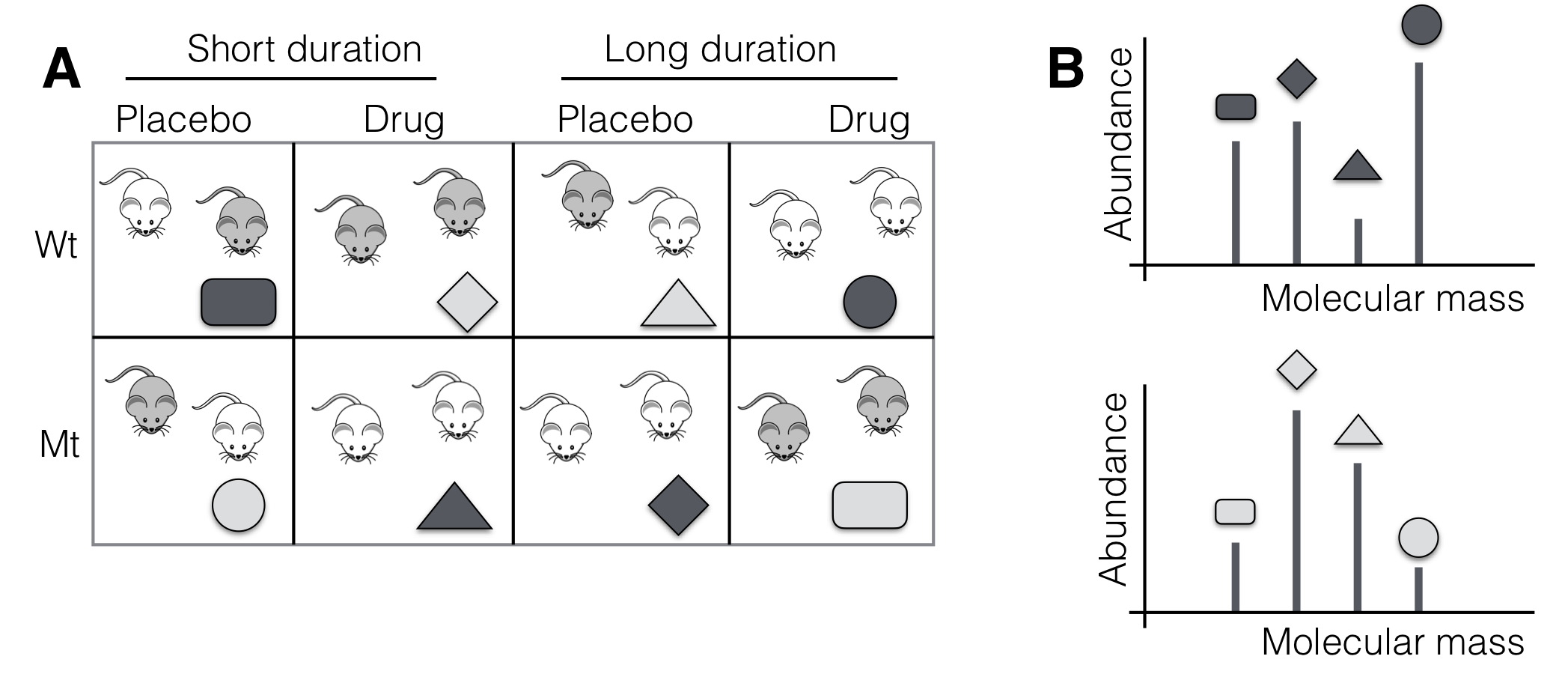
Figure 9.3: Proteomics experiment. A: \(2^3\)-factorial treatment structure with three-way interaction confounded in two blocks. B: Mass spectra with four tags (symbol) for same protein from two blocks (shading). The main disadvantage of this choice is the confounding of the three-way interaction with the block effect, which only allows imprecise estimation, and it is unlikely that the effect sizes are large enough to allow reliable detection in this design. Alternatively, we can use two generators for the two pairs of blocks, the first confounding the three-way interaction, and the second confounding one of the three two-way interactions. A promising candidate is the drug-by-duration interaction, since we are very interested in the genotype-by-drug interaction and would like to detect different activation times between the known and alternative pathways, but we do not expect a drug-by-duration interaction of interest. This yields the data shown in Figure 9.4, where the eight resulting protein abundances are shown separately for short and long duration between drug administration and measurement, and for three typical proteins in the known pathway, in an alternative pathway, and unrelated to the inflammation response. 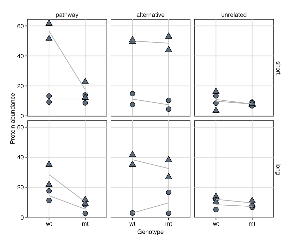
Figure 9.4: Data of proteomics experiment. Round point: placebo, triangle: drug treatment. Panels show typical protein scenarios in columns and waiting duration in rows. 9.9 Notes and SummaryNotesDeliberate effect confounding in factorial designs was fully developed in the 1940s (Fisher 1941; Finney 1945) and is an active research area to this day. A general review is given in Gunst and Mason (2009), and modern developments for multi-stratum designs are given in Cheng (2019). Some specific designs are discussed for engineering applications in Box (1992) and Box and Bisgaard (1993). Fractional factorials can also be constructed for factors with more than two levels, such as the \(3^k\)-series (Cochran and Cox 1957), or generally the \(p^k\)-series (\(p\) a prime number). A more general concept for confounding in factorials with mixed number of factor levels are design keys (Patterson and Bailey 1978). For the analysis of non-replicated designs, the methods by Lenth (Lenth 1989) (discussed in Section 6.4.2) and Box (Box and Meyer 1986) are widely used. The website for NIST’s Engineering Statistics Handbook provides tables with commonly used \(2^{k-l}\)-fractional factorials, Plackett-Burman, and other useful designs in its Chapter 5. Aliasing and the Linear ModelWe provide more details on the aliasing in a half-fraction of the \(2^3\)-factorial design with generic treatment factors A, B, and C, each with levels \(-1\) (low) and \(+1\) (high). The linear model for this design is \[\begin{align*} y_{ijkl} = & \mu + \alpha_A\cdot a_i + \alpha_B\cdot b_j + \alpha_C\cdot c_k \\ & + \alpha_{AB}\cdot a_i\cdot b_j + \alpha_{AC}\cdot a_i\cdot c_k + \alpha_{BC}\cdot b_j\cdot c_k \\ & + \alpha_{ABC}\cdot a_i\cdot b_j\cdot c_k + e_{ijkl}\;, \end{align*}\] where \(a_i\), \(b_j\), \(c_k\) encode the factor level of A, B, and C, respectively for that specific observation. With a sum-encoding, we have \(a_i=-1\) if A is on the low level, and \(a_i=+1\) if A is on the high level, with values for \(b_j\), \(c_k\) accordingly. The seven parameters \(\alpha_X\) are the effects of the corresponding factor that we want to estimate. Using the generator \(ABC=+1\) then translates to imposing the relation \(a_i\cdot b_j\cdot c_k=+1\) for each observation \(i,j,k\), and we can replace \(a_i\cdot b_j\cdot c_k\) with \(+1\) in the linear model equation. It follows that the parameter \(\alpha_{ABC}\) of the three-way interaction is completely confounded with the grand mean \(\mu\). Similarly, we note that \(a_i\cdot b_j = c_k\) for each observation, and we can replace \(a_i\cdot b_j\) with \(c_k\) in the model equation. Thus, the two parameters \(\alpha_{AB}\) and \(\alpha_C\), encoding the effect of the two-way interaction A:B and the main effect of C, respectively, are completely confounded and only their sum \(\alpha_{AB}+\alpha_C\) can be estimated. Continuing this way, we find that the generator implies the linear model \[ y_{ijkl} = \beta_0 + \beta_1 \cdot a_i + \beta_2 \cdot b_j + \beta_3 \cdot c_k + e_{ijkl}\;, \] and we can only estimate its four derived parameters \(\beta_0=\mu+\alpha_{ABC}\), \(\beta_1=\alpha_A+\alpha_{BC}\), \(\beta_2=\alpha_B+\alpha_{AC}\), and \(\beta_3=\alpha_C+\alpha_{AB}\), each parameter corresponding to one alias set. Similarly, the generator \(ABC=-1\) implies that \(a_i\cdot b_j = -c_k\), for example, leading to the four derived parameters \(\gamma_0=\mu-\alpha_{ABC}\), \(\gamma_1=\alpha_A-\alpha_{BC}\), \(\gamma_2=\alpha_B-\alpha_{AC}\), and \(\gamma_3=\alpha_C-\alpha_{AB}\) as the estimable quantities for this half-fraction of the \(2^3\)-factorial design. Using
| ||||||||||||||||||||||||||||||||||||||||||||||||||||||||||||||||||||||||||||||||||||||||||||||||||||||||||||||||||||||||||||||||||||||||||||||||||||||||||||||||||||||||||||||||||||||||||||||||||||||||||||||||||||||||||||||||||||||||||||||||||||||||||||||||||||||||||||||||||||||||||||||||||||||||||||||||||||||||||||||||||||||||||||||||||||||||||||||||||||||||||||||||||||||||||||||||||||||||||||||||||||||||||||||||||||||||||||||||||||||||||||||||||||||||||||||||||||||||||||||||||||||||||