Chapter 8 Split-Unit Designs
8.1 Introduction
In previous designs, we randomized all treatment factors on the same unit factor and these designs therefore have a single experimental unit factor. In some experimental setups, however, some treatment factors are more conveniently applied to groups of units while others can easily be allocated to individual units within groups.
For example, we might study the growth rate of a bacterium at different concentrations of glucose and different temperatures. Using 96-well plates for growing the bacteria, we can use a different amount of glucose for each well, but incubation restricts the whole plate to the same temperature. In other words, a well is the experimental unit for the glucose treatment while a plate is the experimental unit for the temperature treatment.
This kind of design is known as a split-unit (or split-plot) design, where (at least) two treatment factors (glucose concentration and temperature) are randomized on different nested unit factors (plates and wells nested in plates). The precision of a contrast estimate then depends on the treatment factors involved and their respective experimental units.
A related experimental design is the criss-cross design (commonly called split-block or strip-plot), where the two experimental unit factors are crossed rather than nested. This design naturally arises, e.g., when using a multi-channel pipette in a 96-well experiment: with one treatment per channel, all wells in a row of the plate contain the same treatment. Using different concentrations for a dilution series randomized over columns yields the second treatment and experimental unit since all wells in a column have the same dilution.
Both types of designs require care in the model specification to correctly reflect the relations between treatments and units. Otherwise, precision and power are overstated for some contrasts, resulting in deceptively low uncertainties and erroneous conclusions.
8.2 Simple Split-Unit Design
We begin our discussion using two nested unit factors and two crossed treatment factors. A common application of the split-unit design is the accommodation of hard-to-change factors where applying a different level of one treatment factor is much more cumbersome than applying a different level of the other. To avoid frequent simultaneous changes of both levels, we keep the first treatment factor constant for a group of units, and randomize the second treatment factor within this group. This sacrifices precision and power for main effects of the first factor for the benefit of easier implementation. We call the first treatment factor the whole-unit treatment, and the group unit factor the whole-unit. We randomize the second treatment factor (the sub-unit treatment) on the nested unit factor (the sub-unit).
8.2.1 Experiment
We revisit our drug-diet example, with three drugs (placebo, \(D1\), \(D2\)) combined with two diets (low fat, high fat) in an experiment with four mice per treatment, 24 mice in total, using enzyme level as our response.
In previous instances, we randomly assigned a drug-diet combination to each mouse (or each mouse in each block). To implement such an experiment, we have to individually apply the assigned drug to each mouse once at the beginning of the experiment. But we also have to feed each mouse its respective diet throughout the experiment; even if we hold several mice in one cage, we cannot apply the same diet to the whole cage, but have to individually feed each mouse within each cage.
A more practical implementation of the experiment uses eight cages with three mice, but while each mouse per cage is treated with a different drug, all mice in the same cage are fed the same diet. This makes each cage a block for the drugs, but the experimental unit for the diets. The experimental layout is shown in Figure 8.1.
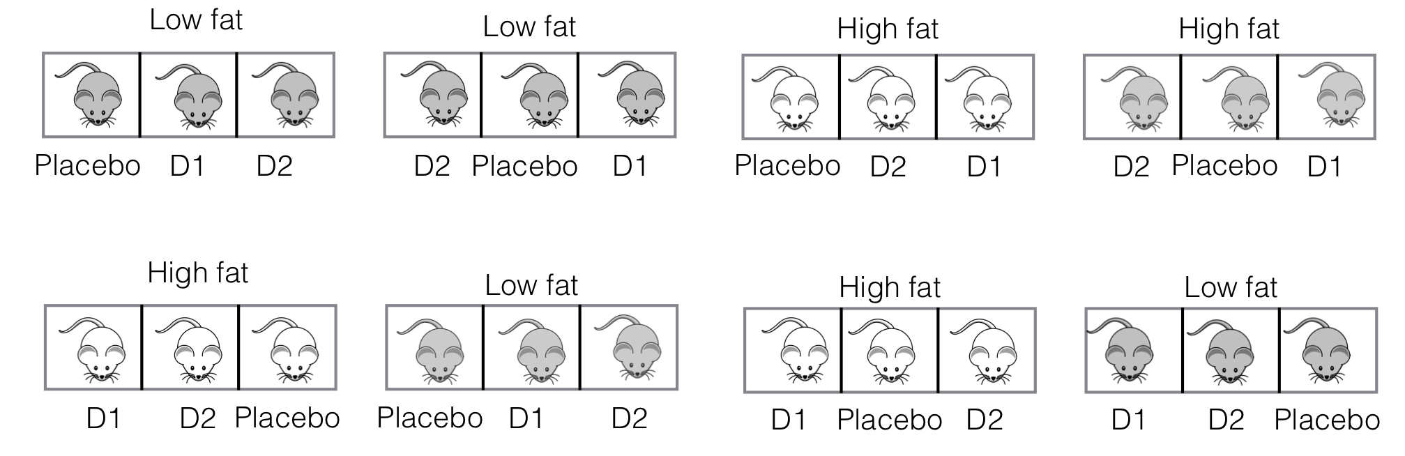
Figure 8.1: Split-unit experiment with two diets randomized on cages of three mice, and three drugs randomized on mice within cages.
8.2.2 Hasse Diagram
The Hasse diagrams are constructed using our previous approaches and are shown in Figure 8.2. The treatment structure is a \(3\times 2\) factorial with interaction. The unit structure consists of (Mouse) (quite literally) nested in (Cage); since we measure one sample per mouse, (Mouse) is the response unit.
In contrast to previous designs, the two treatment factors now have different experimental units: we feed all mice in a cage the same diet, and Diet is randomized on (Cage), while Drug is randomized on (Mouse). Each level of the interaction Diet:Drug is a combination of a diet and a drug, and is randomly assigned to a mouse. As for most blocked designs, we assume that interactions between unit and treatment factors are negligible and do not include the factors (Cage:Drug) and (Cage:Diet:Drug).
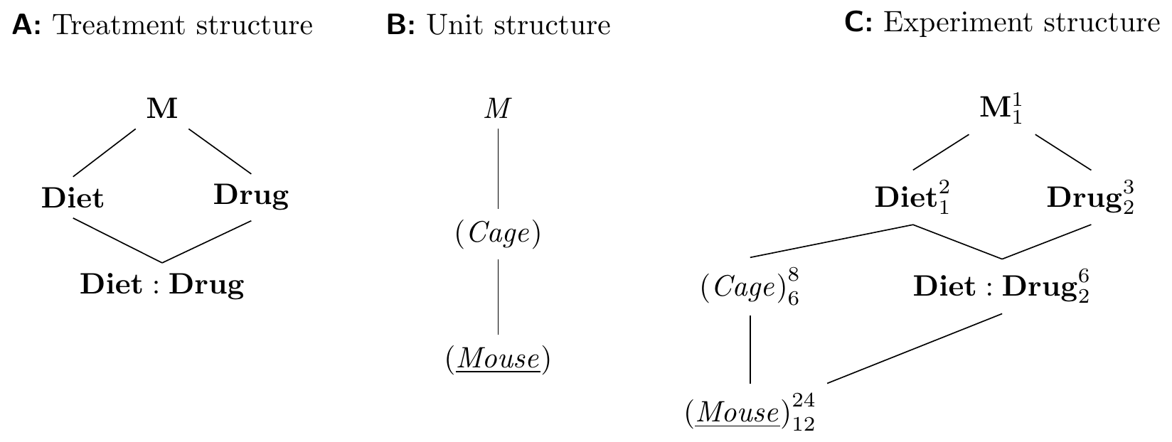
Figure 8.2: Split-unit design with diets randomized on cages and drugs randomized on mice within cages. Cages are blocks for the drug treatment, but experimental units for the diet treatment.
The experiment design diagram shows that (Cage) is a blocking factor for Drug and Drug:Diet; this removes the between-cage variation for contrasts of drug main effects and drug-diet interactions, but not for contrasts involving only Diet. Likewise, the presence of more than one mouse per cage looks like pseudo-replication for diet main effects, and increasing the number of mice per cage does not increase replication for Diet.
The \(F\)-test and contrasts for Diet are based on the degrees of freedom and the variation associated with (Cage). Power and precision are therefore lower than for Drug and Drug:Diet, whose \(F\)-tests and contrasts are based on (Mouse). The loss of precision for the whole-unit factor is the principal disadvantage of a split-unit design. For our purposes, the design is still successful: first, it achieves the desired simplified implementation of the experiment. Second, our main research question concerns the effects of the three drugs (the Drug main effect) and their modification by the diet (the Drug:Diet interaction). Both are based on the full replication and the lowest residual variance terms in the design. We are not interested in comparing only the diets themselves and our intended analysis is therefore largely unaffected by the comparatively low replication and precision for the Diet main effect.
The linear model for this design is \[ y_{ijk} = \mu + \alpha_i + \beta_j + (\alpha\beta)_{ij} + c_{jk} + e_{ijk}\;, \] where \(\alpha_i\), \(\beta_j\), \((\alpha\beta)_{ij}\) are the drug and diet main effect parameters and the interaction parameters with \(i=1\dots 3\) and \(j=1\dots 2\). The random variables \(c_{jk}\sim N(0,\sigma_c^2)\) are effects for the eight cages, and \(e_{ijk}\sim N(0,\sigma_e^2)\) are the residuals within each cage with \(k=1\dots 4\).
8.2.3 Analysis of Variance
We derive the model specification directly from the experiment design diagram (Fig. 8.2C). All random factors are present in the unit structure, and the Error() term is therefore Error(cage/mouse) or simply Error(cage). The fixed factors are all in the treatment structure, which is specified as drug*diet. The model specification is hence y~drug*diet+Error(cage), leading to an ANOVA table with two error strata. We find each treatment factor exclusively in the error stratum of its experimental unit: Diet appears in the (Cage) error stratum and Drug and the interaction appear in the residual (Mouse) error stratum. The correct denominator for each \(F\)-test is found by starting from the corresponding treatment factor in the diagram, and following the edges downward until we find the first random factor: Diet is tested against the variation from cage to cage alone, and the \(F\)-test is based on one numerator and six denominator degrees of freedom. The resulting ANOVA table is:
| Df | Sum Sq | Mean Sq | F value | Pr(>F) | |
|---|---|---|---|---|---|
| Error stratum: Cage | |||||
| diet | 1 | 4.5 | 4.5 | 2.01 | 2.07e-01 |
| Residuals | 6 | 13.47 | 2.24 | ||
| Error stratum: Within | |||||
| drug | 2 | 47.11 | 23.55 | 26.17 | 4.21e-05 |
| drug:diet | 2 | 11.2 | 5.6 | 6.22 | 1.40e-02 |
| Residuals | 12 | 10.8 | 0.9 | ||
Comparing the degrees of freedom in this table with those from the diagram confirms that our model specification corresponds to the design. Between-cage variation seems to be the dominant source of random variation in this experiment, and we are unable to detect any significant main effect for Diet. Both Drug and Drug:Diet are tested against the lower within-cage variation on twelve degrees of freedom, resulting in higher power.
8.2.4 Linear Mixed Model
An equivalent analysis using the linear mixed model uses the specification y~drug*diet+(1|cage), where we directly find a between-cage variance of \(\hat{\sigma}_c^2=\) 0.45, which is about half of the residual variance \(\hat{\sigma}_e^2=\) 0.9, leading to an intra-class correlation of ICC=33%. The cages provide less efficient blocking than litters, but this is unproblematic since we introduced this factor to simplify the experiment implementation, and blocking for the drug effects is simply a welcome benefit.
The linear mixed model calculates sums of squares for Diet and (Cage) differently, but \(F\)-values and \(p\)-values are identical to the ANOVA:
| Sum Sq | Mean Sq | NumDF | DenDF | F value | Pr(>F) | |
|---|---|---|---|---|---|---|
| drug | 47.11 | 23.55 | 2 | 12 | 26.17 | 4.21e-05 |
| diet | 1.81 | 1.81 | 1 | 6 | 2.01 | 2.07e-01 |
| drug:diet | 11.2 | 5.6 | 2 | 12 | 6.22 | 1.40e-02 |
The interaction explains about 19% of the variation and its resulting \(F\)-test is statistically significant.
8.2.5 Contrast Analysis
We define and estimate linear contrasts based on a split-unit design in the same way as before, and can rely on estimated marginal means for providing the required treatment group means. Contrasts of drugs and of drug-diet interactions profit from higher replication and lower variance and are more precise than those comparing diets.
As an illustration, we first compare \(D1\) and \(D2\) to the placebo treatment separately under both diets and use a Dunnett-correction for multiple testing:
| Contrast | Diet | Estimate | SE | df | LCL | UCL |
|---|---|---|---|---|---|---|
| D1 - Placebo | low fat | 2.66 | 0.67 | 12 | 0.97 | 4.35 |
| D2 - Placebo | low fat | 3.22 | 0.67 | 12 | 1.53 | 4.91 |
| D1 - Placebo | high fat | 4.07 | 0.67 | 12 | 2.38 | 5.77 |
| D2 - Placebo | high fat | 1.30 | 0.67 | 12 | -0.39 | 2.99 |
Precision decreases for contrasts that involve comparisons between diets, such as contrasting the placebo averages between the two diets:
| Contrast | Estimate | SE | df | LCL | UCL |
|---|---|---|---|---|---|
| Placebo (high) - Placebo (low) | -0.7 | 0.82 | 14.74 | -2.45 | 1.06 |
This contrast had the same precision as the four other contrasts in our previous designs, but has higher standard error and lower precision in this split-unit design.
8.2.6 Inadvertent Split-Unit Designs
The fact that several experimental unit factors are present requires particular care in setting up the analysis, and split-unit experiments are notorious for the many ways they can be incorrectly designed, analyzed, and interpreted. One problem is mis-specification of the model. Starting from the Hasse diagram, this problem is easily avoided and the results can be checked by comparing the degrees of freedom between diagram and ANOVA table.
Another common problem is the inadvertent split-unit design, where an experiment is intended as, e.g., a completely randomized design but implemented as a split-unit design. Examples are numerous, particularly (but by no means exclusively) in the engineering literature on process optimization and quality control.
Inadvertent split-unit designs usually originate in the implementation phase, by deviating from the design table for a more convenient implementation. For example, a technician might realize that feeding mice by cage rather than individually simplifies the experiment, and create a split-unit design out of an anticipated CRD.
8.3 A Historical Example—Oat Varieties
In his classic paper “Complex Experiments,” Frank Yates reviews and expands the advances in statistical design of experiments since the 1920s (Yates 1935). The paper contains an experiment to investigate different varieties of oat using several levels of nitrogen as fertilizer, which we discuss as an additional example of a split-unit design with additional blocking.
The experiment is illustrated in Figure 8.3A: three oat varieties “Victory,” “Golden Rain,” and “Marvellous” (denoted \(v_1\dots v_3\)) are applied to plots of sufficient size. Meanwhile, four nitrogen levels \(n_1\dots n_4\) are applied to smaller patches of land, denoted subplots (nested in plots). This yields a split-unit design with varieties randomized on plots, and nitrogen on subplots nested in plots.
A common problem in agricultural experimentation is the heterogeneity of the soil, exposure to sunlight, irrigation, and other factors, which add substantial variability between plots that are spatially more distant. In this example, the whole experiment is replicated in six blocks \(\text{I}\dots\text{VI}\), where each block consists of three neighboring plots, and varieties are independently randomized to plots within each block. This increases the replication to achieve precision of contrasts between varieties while simultaneously controlling for spatial heterogeneity over a large area. The design is therefore a split-unit design with a randomized complete block design on the whole-plot level.
The resulting 72 observations are shown in Figure 8.3B, individually for each block. Block effects are clearly visible, and patterns are very similar between blocks, so assuming no block-by-treatment interaction seems reasonable. We also observe a pronounced trend of increasing yield with increasing nitrogen level, and this trend seems roughly linear. Differences between oat varieties are less obvious.
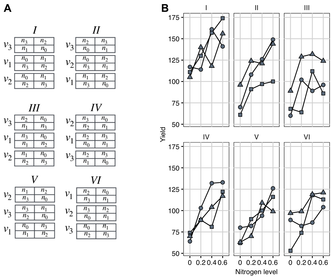
Figure 8.3: A: Split-unit design with three oat varieties randomized on plots, four nitrogen amounts randomized on subplots within plots, and replication in six blocks. B: Data shown separately for each block. Point: Golden Rain; triangle: Marvellous; square: Victory.
The Hasse diagrams are given in Figure 8.4 and show the simple factorial treatment structure and the chain of nested unit factors combined into a fairly complex design, where the whole treatment structure is blocked, and the nitrogen and interaction treatment factors are blocked by the plots.
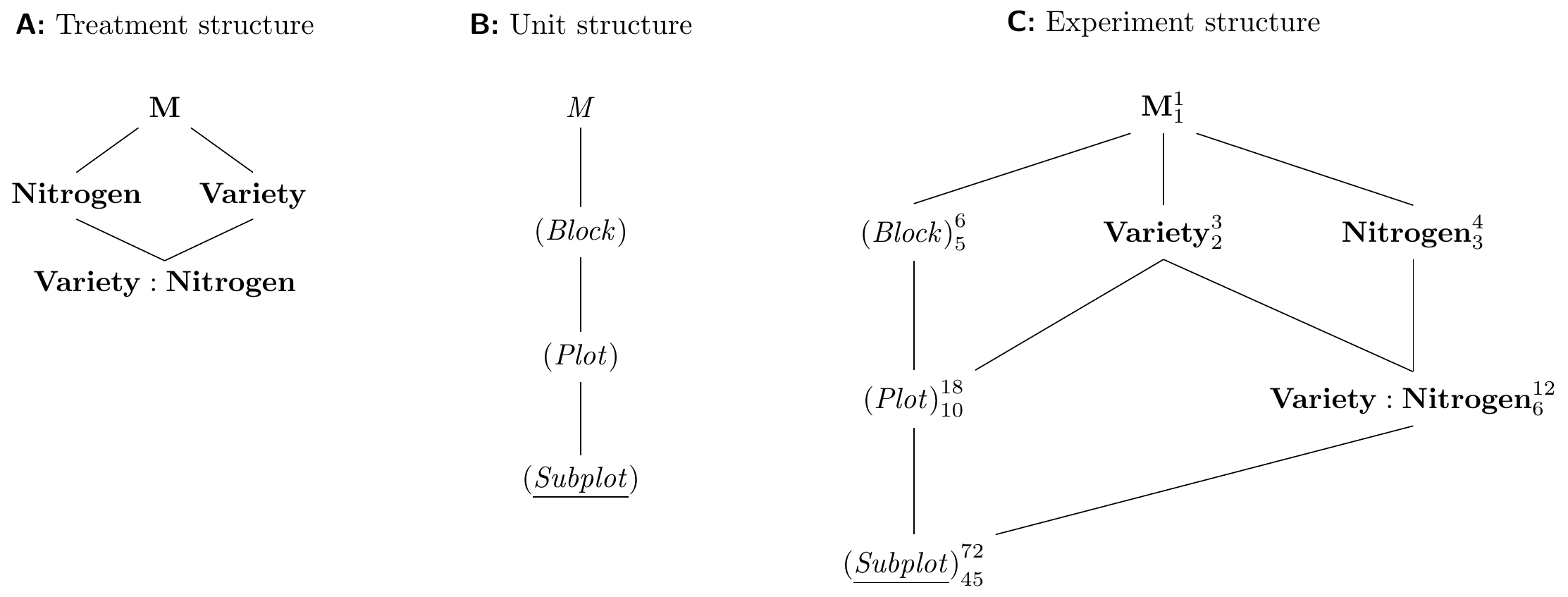
Figure 8.4: Hasse diagram for Yates’ oat variety and nitrogen example with two treatment factors randomized on plots respectively subplots in plots, and replication in six blocks.
The original analysis in 1930 was of course done using an analysis of variance approach. Here, we analyze the experiment using a linear mixed model and derive the specification Variety*Nitrogen+(1|Block)+(1|Plot:Block) from the Hasse diagram. This yields the following ANOVA table:
| Sum Sq | Mean Sq | NumDF | DenDF | F value | Pr(>F) | |
|---|---|---|---|---|---|---|
| Variety | 526.06 | 263.03 | 2 | 10 | 1.49 | 2.72e-01 |
| Nitrogen | 20020.5 | 6673.5 | 3 | 45 | 37.69 | 2.46e-12 |
| Variety:Nitrogen | 321.75 | 53.62 | 6 | 45 | 0.3 | 9.32e-01 |
The small and non-significant interaction shows that increasing the nitrogen level has roughly the same effect on yield for all three oat varieties. In addition, differences between oat varieties are also small with average yields between 80 and 175 and differences all less than 10, and not significant. The nitrogen level, on the other hand, shows a large and highly significant effect, and higher levels give more yield.
We further quantify these findings by estimating corresponding contrasts and their confidence intervals. First, we compare the varieties within each nitrogen level (Table 8.1). In each case, Marvellous provides higher yield than both Golden Rain and Victory, and Golden Rain gives higher yield than Victory: the varieties have a clear order, which is stable over all nitrogen levels. As the confidence intervals show, however, none of the differences are significant, and the precision of estimates is fairly low.
| Contrast | Estimate | se | df | LCL | UCL |
|---|---|---|---|---|---|
| Nitrogen: 0.0 | |||||
| Golden Rain - Marvellous | -6.67 | 9.72 | 30.23 | -30.61 | 17.27 |
| Golden Rain - Victory | 8.50 | 9.72 | 30.23 | -15.44 | 32.44 |
| Marvellous - Victory | 15.17 | 9.72 | 30.23 | -8.77 | 39.11 |
| Nitrogen: 0.2 | |||||
| Golden Rain - Marvellous | -10.00 | 9.72 | 30.23 | -33.94 | 13.94 |
| Golden Rain - Victory | 8.83 | 9.72 | 30.23 | -15.11 | 32.77 |
| Marvellous - Victory | 18.83 | 9.72 | 30.23 | -5.11 | 42.77 |
| Nitrogen: 0.4 | |||||
| Golden Rain - Marvellous | -2.50 | 9.72 | 30.23 | -26.44 | 21.44 |
| Golden Rain - Victory | 3.83 | 9.72 | 30.23 | -20.11 | 27.77 |
| Marvellous - Victory | 6.33 | 9.72 | 30.23 | -17.61 | 30.27 |
| Nitrogen: 0.6 | |||||
| Golden Rain - Marvellous | -2.00 | 9.72 | 30.23 | -25.94 | 21.94 |
| Golden Rain - Victory | 6.33 | 9.72 | 30.23 | -17.61 | 30.27 |
| Marvellous - Victory | 8.33 | 9.72 | 30.23 | -15.61 | 32.27 |
For quantifying the dose-response relationship between nitrogen level and yield, we estimate the nitrogen main effect contrasts independently within each oat variety. We use a polynomial contrast for Nitrogen, which provides information about linear, quadratic, and cubic components of a dose-response. The results are shown in Table 8.2.
| Contrast | Estimate | se | df | t value | P(>|t|) |
|---|---|---|---|---|---|
| Golden Rain | |||||
| linear | 150.67 | 24.30 | 45 | 6.20 | 0.00 |
| quadratic | -8.33 | 10.87 | 45 | -0.77 | 0.45 |
| cubic | -3.67 | 24.30 | 45 | -0.15 | 0.88 |
| Marvellous | |||||
| linear | 129.17 | 24.30 | 45 | 5.32 | 0.00 |
| quadratic | -12.17 | 10.87 | 45 | -1.12 | 0.27 |
| cubic | 14.17 | 24.30 | 45 | 0.58 | 0.56 |
| Victory | |||||
| linear | 162.17 | 24.30 | 45 | 6.67 | 0.00 |
| quadratic | -10.50 | 10.87 | 45 | -0.97 | 0.34 |
| cubic | -16.50 | 24.30 | 45 | -0.68 | 0.50 |
For each variety, we find a substantial linear upward trend. Since both quadratic and cubic terms are small and not significant, we can ignore all potential curvature in the trends and arrive at an easy to interpret result: the yield increases proportionally with increases in nitrogen level. We already determined that the average and nitrogen-level-specific yields are almost identical between varieties. The current contrasts additionally show that the estimates of the three linear components are all within roughly one standard error of each other, demonstrating a comparable dose-response relation for all three varieties. This of course agrees with the previous result that there is no variety-by-nitrogen interaction.
8.4 Variations and Related Designs
The split-unit design turns out to be quite ubiquitous in experimental work. We briefly discuss several variations of this design idea to explore some additional uses: accommodating an additional factor in an already existing design, using more than two nested units and randomizing a treatment factor on each level of nesting, and using crossed rather than nested experimental units for the treatment allocation. We also introduce the simplest case of cross-over designs, where two treatments are used in sequence on the same experimental unit. Finally, longitudinal experimental designs involving a (usually temporal) order of treatments and measurements such as for comparing a response before and after application of a treatment are sometimes considered and analyzed as split-unit designs.
8.4.1 Accommodating an Additional Factor
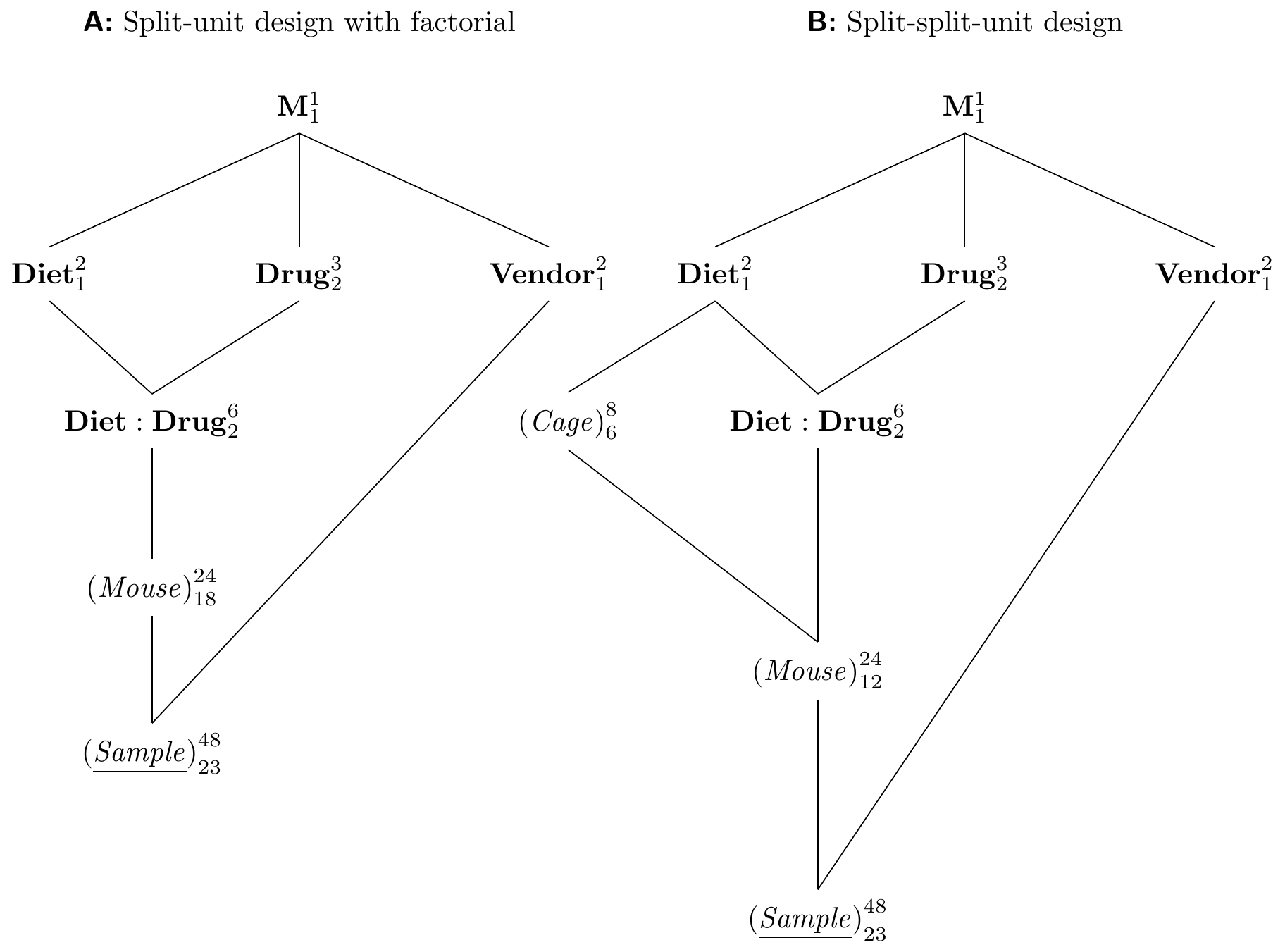
Figure 8.5: A: Split-unit design with diets and drugs completely randomized on mice as a CRD and vendor randomized on samples. B: Same treatment structure with split-split-unit design.
We turned our previous drug-diet example into a split-unit design by grouping mice into cages and using the new grouping factor as experimental unit for the diets. This creates a whole-plot factor ‘above’ the original experimental unit. Similar to our discussion of choosing a blocking factor for an RCBD, we can alternatively sub-divide the original experimental unit further to create a sub-plot factor ‘below.’
To illustrate this idea, we consider the following situation: we start from our original drug-diet design with factorial treatment structure randomized on mice (a CRD). Previously, we also considered comparing two sample preparation kits from vendors A and B based on the enzyme level measurements. Since we already have our drug-diet experiment planned, we would like to ‘squeeze’ the comparison of the two kits into that experiment without jeopardizing our main objective of estimating contrasts of the drug-diet treatments.
The idea is simple: we draw two samples per mouse and randomly assign either kit A or kit B to each sample. The resulting experiment structure is shown in Figure 8.5A and we recognize it as a split-unit design. Here, the whole-plot unit (Mouse) is combined with a factorial treatment structure, and the sub-plot unit (Sample) is nested in (Mouse) to compare levels of Vendor. The resulting treatment structure is a \(3\times 2\times 2\) factorial, where we removed all interactions involving Vendor under the assumption that these are negligible. The original drug-diet experiment is then unaffected by this augmentation of the design: even if vendor B’s kit is worse, we still have the full data for vendor A; simply removing the B data yields the data for the originally anticipated design.
We use the linear mixed model framework for estimating the corresponding model with specification y~drug*diet+vendor+(1|mouse) and estimating the difference between the two vendors.
| Contrast | Estimate | se | df | LCL | UCL |
|---|---|---|---|---|---|
| Vendor A - Vendor B | -0.4 | 0.18 | 23 | -0.77 | -0.02 |
This contrast is estimated very precisely with 23 residual degrees of freedom, the same as for a randomized complete block design with 24 mice as blocks and two samples per mouse and no other treatment factors. It has much higher precision than the drug or diet comparisons, because each mouse provides a block for Vendor to compare the two kits within each mouse.
8.4.2 Split-Split-Unit Designs
By introducing three nested unit factors and randomizing one treatment factor on each, we arrive at a split-split-unit design. Further extensions to arbitrary levels of nested factors are straightforward.
For example, we combine the split-unit design for drugs and diets with a comparison of the two vendors. The new design is shown in Figure 8.5B and uses (Cage) as experimental unit for the hard-to-change factor Diet, (Mouse) in (Cage) as experimental unit for Drug, and (Sample) in (Mouse) in (Cage) to accommodate Vendor as an additional treatment factor.
From the diagram, we find one random intercept for each cage, leading to a random effect term (1|cage), one random intercept for each mouse within a cage, with (1|cage:mouse), and the omitted (1|cage:mouse:sample). A linear mixed model that ignores all interactions of Vendor with other factors is therefore specified as y~drug*diet+vendor+(1|cage)+(1|cage:mouse) and yields the ANOVA table
| Sum Sq | Mean Sq | NumDF | DenDF | F value | Pr(>F) | |
|---|---|---|---|---|---|---|
| drug | 26.29 | 13.15 | 2 | 12 | 33.44 | 1.24e-05 |
| diet | 1.02 | 1.02 | 1 | 6 | 2.6 | 1.58e-01 |
| vendor | 1.89 | 1.89 | 1 | 23 | 4.81 | 3.87e-02 |
| drug:diet | 4.51 | 2.26 | 2 | 12 | 5.74 | 1.78e-02 |
The results are very similar to our split-unit design without the additional Vendor treatment. Interactions involving Vendor can of course be introduced, and lead to a more complex analysis and interpretation of results.
8.4.3 Criss-Cross or Split-Block Designs
In contrast to the split-unit design, we cross the two unit factors in a criss-cross design and combine this unit structure with a factorial treatment structure. The simplest instance of a criss-cross design is a row-column design with \(a\) rows and \(b\) columns, where a treatment factor with \(a\) levels is randomized on the rows, and a crossed treatment factor with \(b\) levels is randomized on columns. This treatment structure is an \(a\times b\) factorial, but each treatment factor has its own experimental unit. In contrast to a split-unit design, the interaction of the two treatment factors does not share its experimental unit with any of the main effect factors. For a two-way factorial treatment structure, the criss-cross design therefore has three experimental units and such a design needs to be replicated several times to arrive at suitable residual degrees of freedom for all experimental unit factors. Usually, the rows and columns are independently replicated, and randomization is done independently for each replicate of the row-column criss-cross design.
Example: Multi-Channel Pipetting
The criss-cross design rather naturally arises in experiments on 96-well plates when using multi-channel pipettes; common multi-channel pipettes offer eight channels such that eight consecutive wells can be handled simultaneously.
This setup is advantageous in assays based on dilution series, where up to eight different conditions are subjected to twelve dilutions each. A typical response is the optical density in each well, for example. Using one pipette channel for each condition allows randomization of the conditions on the rows of each plate, but the same condition is then assigned to all wells in the same row. Similarly, the dilution steps can be randomized on columns, but each of the eight rows then has a fixed dilution. This arrangement leads to a criss-cross design with conditions randomized on rows by randomly assigning them to the channels of the pipette at the beginning of the experiment, and dilutions randomized on columns.
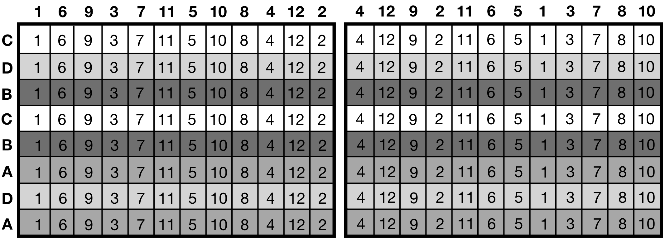
Figure 8.6: Criss-cross experiment layout: two replicates of four drugs (background shade) randomized on rows, dilutions (numbers) randomized on columns. Two replicate plates shown, randomization of rows kept constant while dilutions are randomized independently.
The plate layouts in Figure 8.6 show a version of this strategy for comparing the effect of four drugs on bacterial growth in twelve glucose concentrations in the growth medium. Two channels are randomly assigned to each drug and each glucose level is used on one full column; we use two plates to provide higher replication. For easier implementation, the assignment of drugs to pipette channels is only randomized once, and then kept identical for both plates. The glucose levels are randomized independently to columns for each plate. This provides an interesting variant of the criss-cross design.
The Hasse diagrams for this example are shown in Figure 8.7. The treatment structure is a simple two-way factorial design of drug and glucose. In the unit structure, columns are nested in plates since randomization is independent between plates, but rows are crossed with plates since any row in the first plate is identified with the corresponding row in the second plate. We omitted several interaction factors that we assume negligible for brevity, but the experiment structure is already rather complex.
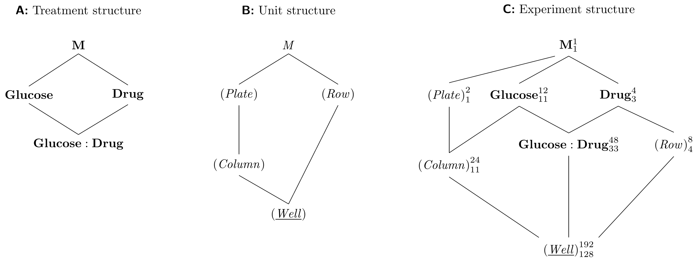
Figure 8.7: Criss-cross design arising from use of multichannel pipette. Four drugs are tested with 12 glucose concentrations on each plate, two plates provide replication. Use of 8-channel pipette allows two replicates of each drug; random assignment of drug to channel is kept constant for both plates, but assignment of glucose concentration to columns is randomized independently.
From the experiment diagram, we derive the model specifications y ~ drug * glucose + Error(plate/col + row) for an ANOVA and y ~ drug * glucose + (1|plate/col) + (1|row) for a linear mixed model. The classical ANOVA table has four error strata: one for (Plate), one for (Column) in (Plate) containing the Glucose main effect, one for (Row) containing the Drug main effect, and the residual error stratum containing the Glucose:Drug interaction. The linear mixed model provides direct estimation of the four variances in this model, and its ANOVA table is
| Sum Sq | Mean Sq | NumDF | DenDF | F value | Pr(>F) | |
|---|---|---|---|---|---|---|
| drug | 30.35 | 10.12 | 3 | 4 | 6.32 | 5.35e-02 |
| glucose | 38.7 | 3.52 | 11 | 11 | 2.2 | 1.04e-01 |
| drug:glucose | 46.82 | 1.42 | 33 | 128 | 0.89 | 6.47e-01 |
The denominator of the three treatment \(F\)-tests corresponds to the closest random factor below its treatment factor. With several random factors crossed and nested, traditional ANOVA and linear mixed model results differ; we would prefer the latter.
8.4.4 Cross-Over Designs
A useful design for increasing precision and power is the cross-over design, where different treatments are assigned in sequence to the same experimental unit. As a basic example, we consider an experiment for determining the effect of the low- and high fat diet (with no drug treatment) on the enzyme levels. We use six mice, which we split into two groups: we feed the mice in the first group on the low fat diet for some time, and then switch them to the high fat diet. In the second group, we reverse the order and feed first the high fat diet, and then the low fat diet. This is a two-period two-treatment cross-over design. The experiment is illustrated in Figure 8.8 for three mice per group.
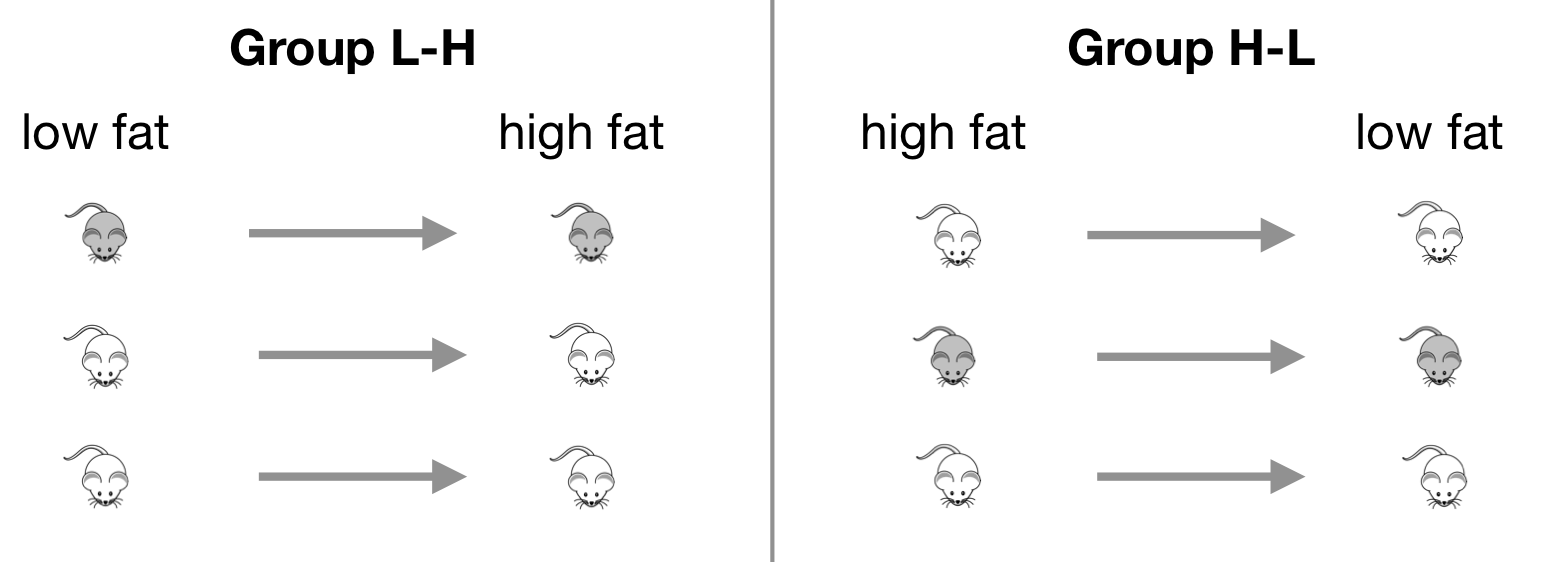
Figure 8.8: Cross-over experiment with two diets assigned in one of two orders.
Before each diet treatment, we feed all mice with a standard diet. This should allow the enzyme level to reset to ‘normal,’ such that the first diet does not affect observations with the second diet. The observations are taken after several days on the respective diet, with one observation per mouse per diet.
The experiment diagram is shown in Figure 8.9A. The treatment factor Sequence denotes the group: each mouse is assigned to either the low-high (L-H) sequence of diets, or the high-low (H-L) sequence. The sequence is crossed with the second treatment factor Diet, since each diet occurs in each sequence. Each level of the interaction Sequence:Diet corresponds to the application of one diet at a specific part in each sequence (the period). Each mouse is randomly assigned to one sequence, so (Mouse) is the experimental unit for Sequence. Each sample corresponds to a combination of a period and a diet, and is the experimental unit for Diet and the interaction.
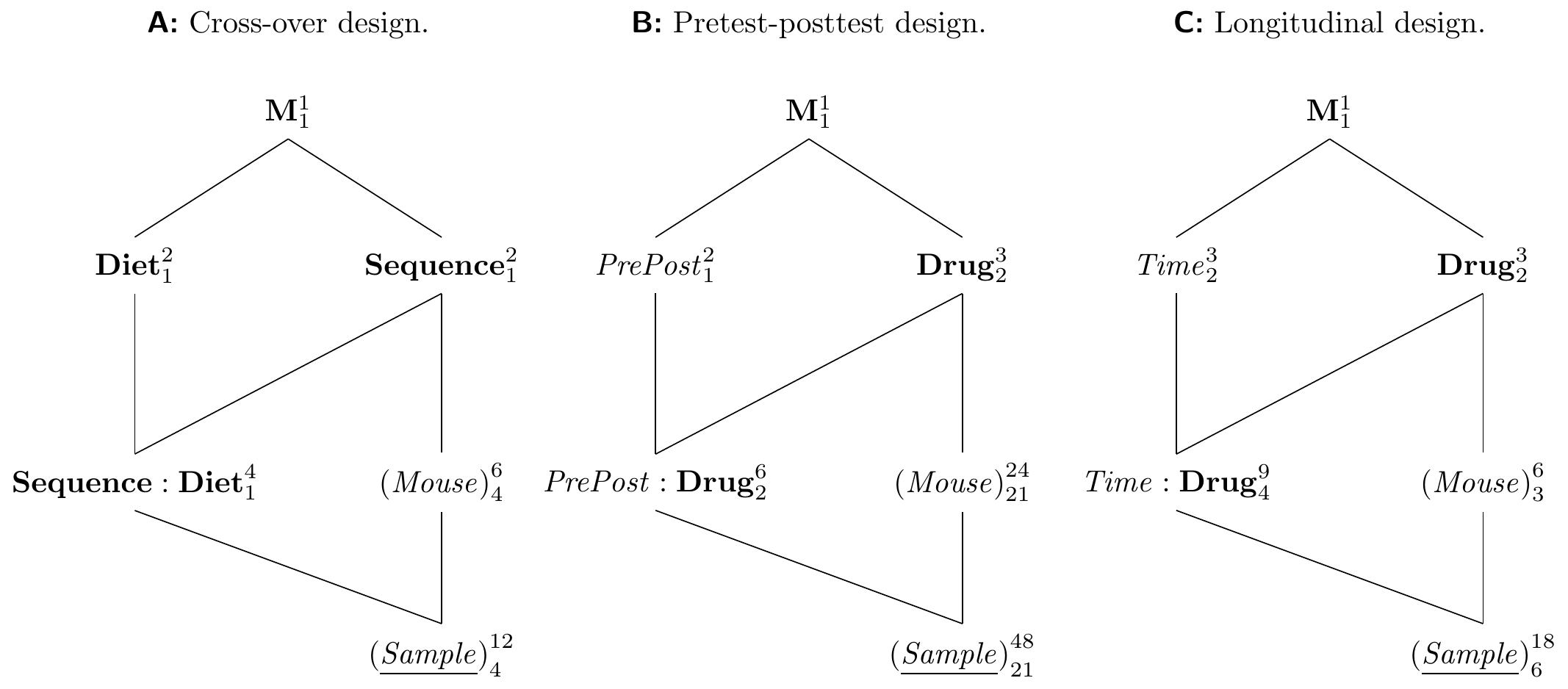
Figure 8.9: A: Cross-over design uses two diet treatments sequentially on same mouse to provide within-mouse contrasts. B: Pretest-posttest design with measurement before and after application of treatment to consider mouse-specific baseline response values. C: Longitudinal repeated measures design to allow multiple measurements of same mouse at different time-points.
It is instructive to consider the effects associated with Sequence, Diet, and Sequence:Diet. Since each factor has one degree of freedom, these effects are simple differences. A commonly used model for a two-period two-treatment cross-over design yields the following expected values for the four period-diet combinations: \[\begin{align*} \mu_{LH1} &= \mu+\alpha_L+\pi_1 && \text{(low-high, first observation)}\\ \mu_{LH2} &= \mu+\alpha_H+\gamma_L+\pi_2 && \text{(low-high, second observation)}\\ \mu_{HL1} &= \mu+\alpha_H+\pi_1 && \text{(high-low, first observation)}\\ \mu_{HL2} &= \mu+\alpha_L+\gamma_H+\pi_2 && \text{(high-low, second observation)}\;, \end{align*}\] where \(\mu\) is the grand mean, \(\alpha_i\) are the effects of the low and high fat diet, \(\pi_j\) is the effect of period \(j\), and \(\gamma_k\) are the residual carry-over effects from the previous diet not eliminated by the washout period between diets.
The Sequence main effect is \[ \frac{1}{2}\left(\mu_{LH1}+\mu_{LH2}\right)-\frac{1}{2}\left(\mu_{HL1}+\mu_{HL2}\right) = \frac{1}{2}(\gamma_L-\gamma_H)\;, \] with associated hypothesis \(H_0:\gamma_L=\gamma_H\) that the two carry-over effects are equal (but not necessarily zero!). This test essentially asks if there is a difference between the two orders in which the diets are applied. If both carry-over effects are equal, then no difference exists since then \(\gamma_L=\gamma_H=\gamma\), and we can merge \(\gamma\) with the period effect \(\pi_2\) (all observations are higher or lower by the same amount in the first compared to the second period).
The Diet main effect is \[ \frac{1}{2}\left(\mu_{LH1}+\mu_{HL2}\right)-\frac{1}{2}\left(\mu_{HL1}+\mu_{LH2}\right) = \alpha_L-\alpha_H-\frac{1}{2}(\gamma_L-\gamma_H)\;, \] and is biased if the two carry-over effects are not equal. Note that we can in principle estimate and test the bias from the Sequence main effect, but that this effect has lowest replication in the design, and low precision and power. In the case of unequal carry-over effects, one often restricts the analysis to data from the first period alone, and estimates the treatment effect via \((\mu_{LH1}-\mu_{HL1})/2\).
The Sequence:Diet interaction effect is \[ \frac{1}{2}\left(\mu_{LH1}-\mu_{LH2}\right)-\frac{1}{2}\left(\mu_{HL1}-\mu_{HL2}\right) = \pi_1-\pi_2-\frac{1}{2}(\gamma_L+\gamma_H)\;, \] and is biased whenever there are—even equal—carry-over effects.
Cross-over designs form an important class of designs and the two-period two-treatment design is only the simplest instance. It does not allow estimation of the carry-over effects, which is a major weakness in practice where carry-over can often be suspected and the experiment should provide information about its magnitude. Better variants of the cross-over design that allow explicit estimation of the carry-over should therefore be preferred whenever feasible. One variant also uses two periods, but includes the two combinations H-H and L-L in addition to H-L and L-H. Carry-over can then be estimated by comparing the H-H to the L-H observations, for example. Another variant extends the design to three periods, with treatment sequences including H-H-L and L-H-L, for example, such that one treatment is observed twice in each sequence. The references in Section 8.5 provide more in-depth coverage of different cross-over designs and associated analyses.
8.4.5 Pretest-Posttest Designs
Another common technique to increase precision is the pretest-posttest design, where the response variable is measured once before and once after the treatment is applied. This provides a simple way for adjusting the treatment response by a subject-specific baseline, and the difference between response after treatment and baseline is then considered as the relevant quantity for estimating the treatment effect. We study a simple example of a pretest-posttest design with a single treatment factor, but the ideas readily extend to factorial treatment structures as well.
We consider our experiment for comparing three drugs, and use the baseline enzyme levels of each mouse in conjunction with the enzyme level after administration of the drug. The experiment diagram in Figure 8.9B illustrates this design. It contains three unit factors, (Sample) nested in (Mouse), since we take two samples from each mouse, one before, one after the drug administration, and the fixed unit factor PrePost, which designates if a sample was taken before or after treatment is administered. The design contains Drug as the only treatment factor, crossed with PrePost. We introduce their interaction as a third factor into the design. Since both samples belong to the same mouse, and a drug is applied to a mouse after the baseline measurement is taken, (Mouse) is the experimental unit for Drug. The corresponding models are y ~ prepost * drug + Error(mouse) for aov(), and y ~ prepost * drug + (1|mouse) for lmer(). Note that while this design looks very similar to a cross-over design, only one treatment is assigned to each mouse and sample.
Because the unit factor PrePost is fixed, there are three \(F\)-tests: the PrePost main effect compares the average response over all drugs before and after administration. We expect that the measured enzyme levels are not systematically different between the three drug groups before applying the treatment. Thus, a small and non-significant pre-post main effect either indicates that the before and after responses are identical for all drugs; none of the drugs has any discernible effect. Or it might be that one drug increases the enzyme level, and another drug decreases it, and the two effects cancel out.
The \(F\)-test of the Drug main effect tests if the average enzyme levels are identical for all three drugs, when before and after measurements are lumped together. The denominator mean squares for this test stem from the between-mouse variation. This test is the least powerful, but also the least interesting.
Of greatest interest is usually the PrePost:Drug interaction, which shows how different the changes of enzyme levels are between drugs from baseline to post-treatment measurement. This is the drug effect corrected for the baseline measurement. We can replicate the corresponding \(F\)-test as follows: for each mouse \(i\), calculate the difference \(\Delta_i=y_{i,\text{post}}-y_{i,\text{pre}}\) of the post-treatment response and the pre-treatment response. This ‘adjusts’ the response to the treatment for the baseline value. Now, we perform a one-way ANOVA with Drug as the treatment factor, and \(\Delta_i\) as the response variable. The resulting \(F\)-ratio and \(p\)-value are identical to the PrePost:Drug test.
8.4.6 Longitudinal Designs
Split-unit designs are sometimes still used for repeated measures and longitudinal designs, in which multiple response variables are measured for the same experimental unit, respectively the same response variable is measured at multiple occasions for the same experimental unit. Both designs thus have a more complex response structure than the classical approach can handle.
An example of a longitudinal design is shown in Figure 8.9C, where three drugs are randomized on two mice each, and each mouse is then measured at three time-points. In this design, we randomize Drug on (Mouse), and the fixed unit factor Time groups the samples from each mouse. We can then relate observations from the same mouse to each other to analyze the temporal profile of each mouse. The advantage of the longitudinal design is that observations can be contrasted within each mouse, and the between-mouse variation is removed from such contrasts.
The main caveat of this approach is the crude approximation of the complex longitudinal response structure by a fixed block factor Time. This assumes that any pair of time-points has the same correlation, while observations closer in time often tend to have stronger correlations than those further apart. This caveat does not apply to the pretest-posttest designs, where only two time-points are considered.
8.5 Notes and Summary
Notes
Insightful accounts on split-unit designs are Federer (1975) and Box (1996), and a gentle introduction is given in Kowalski and Potcner (2003). Recent developments in split-unit designs are reviewed in Jones and Nachtsheim (2009). Analysis of split-unit designs with more complex whole-unit and sub-unit treatment designs are discussed in Goos and Gilmour (2012), and power analysis in Kanji and Liu (1984). Increasing availability of liquid-handling robots renewed interest in split-unit and criss-cross designs for microplate-based experiments (Buzas, Wager, and Lansky 2011).
Different variants of cross-over designs are discussed in detail in Johnson (2010) and Senn (1994), and a tutorial framing the analysis of cross-over designs into linear contrasts is Shuster (2017). A standard text for cross-over designs in clinical trials is Senn (2002), and applications to bioassays were highlighted already in the 1950s (Finney 1956).
An extensive treatment of pretest-posttest designs is Bonate (2000), and an illustrative example comparing two surgical techniques with several different analysis techniques is given in Brogan and Kutner (1980).
The use of split-unit-like designs for longitudinal experiments usually requires analysis techniques with non-sphericity corrections that account for unequal correlation between pairs of observations in the same group (Abdi 2010; Huynh and Feldt 1976; Greenhouse and Geisser 1959). By now, more appropriate models—including more complex variants of the linear mixed model—are available and should be preferred (Fitzmaurice, Laird, and Ware 2011; Diggle et al. 2013).
Using R
The function design.split() generates and randomizes split-unit designs; the option design= allows a CRD, RCBD, or latin squares design for the whole-unit stratum. Criss-cross designs are generated and randomized by the function design.strip(). Both functions are from the agricolae package.
The biggest difficulty in using split-unit designs in R is usually the model specification; this problem is largely alleviated when using Hasse diagrams, from which the specification is directly derived.
Summary
Split-unit designs offer flexibility in the implementation of an experiment when some treatment factors are more conveniently randomized on units that serve as blocks for other treatment factors. The former are sometimes called hard-to-change factors, particularly in the engineering literature. In laboratory work, split-unit designs are often required when different experimental conditions are examined on a 96-well plate, for example, but factors like temperature or shaking frequency apply to the plate as a whole.
With two experimental unit factors, sub-unit treatments have higher replication and are more precisely estimated than whole-unit treatment effects; importantly, however, their interaction also profits from high replication and high precision.
Several common designs such as cross-over designs can be seen as split-unit designs in disguise. Longitudinal designs, including the pretest-posttest design, are sometimes treated as split-unit designs; as an important conceptual difference, however, the whole-unit treatment is replaced by a fixed unit factor to capture the more complex response structure.