Chapter 6 Multiple Treatment Factors: Factorial Designs
6.1 Introduction
The treatment design in our drug example contains a single treatment factor, and one of four drugs is administered to each mouse. Factorial treatment designs use several treatment factors, and a treatment applied to an experimental unit is then a combination of one level from each factor.
While we analyzed our tumor diameter example as a one-way ANOVA, we can alternatively interpret the experiment as a factorial design with two treatment factors: Drug with three levels ‘none,’ ‘CP,’ and ‘IFF,’ and Inhibitor with two levels ‘none’ and ‘RTV.’ Each of the six previous treatment levels is then a combination of one drug and absence/presence of RTV.
Factorial designs can be analyzed using a multi-way analysis of variance—a relatively straightforward extension from Chapter 4—and linear contrasts. A new phenomenon in these designs is the potential presence of interactions between two (or more) treatment factors. The difference between levels of the first treatment factor then depends on the level of the second treatment factor and greater care is required in the interpretation.
6.2 Experiment
In Chapter 4, we suspected that the four drugs might show different effects under different diets, but ignored this aspect by using the same low fat diet for all treatment groups. We now consider the diet again and expand our investigation by introducing a second diet with high fat content. We previously found that drugs \(D1\) and \(D2\) from class A are superior to the two drugs from class B, and therefore concentrate on class A exclusively. In order to establish and quantify the effect of these two drugs compared to “no effect,” we introduce a control group using a placebo treatment with no active substance to provide these comparisons within our experiment.
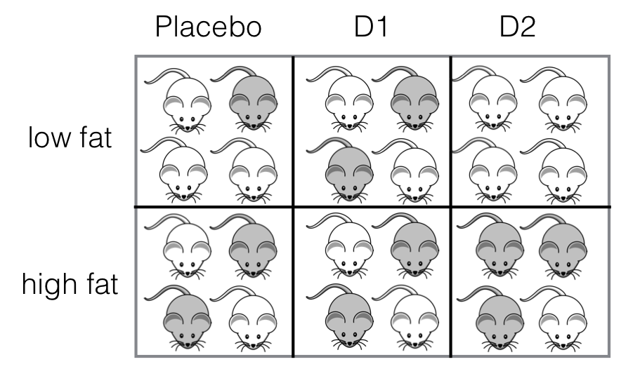
Figure 6.1: Experiment with two crossed treatment factors with four mice in each treatment combination.
The proposed experiment is as follows: two drugs, \(D1\) and \(D2\), and one placebo treatment are given to 8 mice each, and treatment allocation is completely at random. For each drug, 4 mice are randomly selected and receive a low fat diet, while the other 4 mice receive a high fat diet. The treatment design then consists of two treatment factors, Drug and Diet, with three and two levels, respectively. Since each drug is combined with each diet, the two treatment factors are crossed, and the design is balanced because each drug-diet combination is allocated to four mice (Figure 6.1).
| 1…2 | 2…3 | 3…4 | 4…5 | 1 | 2 | 3 | 4 | |
|---|---|---|---|---|---|---|---|---|
| Placebo | 10.12 | 8.56 | 9.34 | 8.70 | 10.79 | 12.01 | 9.11 | 10.71 |
| D1 | 14.32 | 13.58 | 14.81 | 13.98 | 14.08 | 13.86 | 13.94 | 16.36 |
| D2 | 13.61 | 13.24 | 10.35 | 13.31 | 9.84 | 8.84 | 12.04 | 8.58 |
The 24 measured enzyme levels for the six treatment combinations are shown in Table 6.1 and Figure 6.2A. A useful alternative visualization is an interaction plot as shown in Figure 6.2B, where we show the levels of Diet on the horizontal axis, the enzyme levels on the vertical axis, and the levels of Drug are represented by point shape. We also show the average response in each of the six treatment groups and connect those of the same drug by a line, linetype indicating the drug.
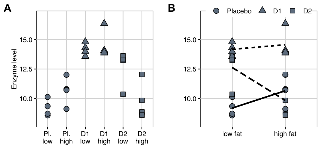
Figure 6.2: A: Enzyme levels for combinations of three drugs and two diets, four mice each in a completely randomized design with two-way crossed treatment structure. Drugs are highlighted as point shapes. B: Same data as interaction plot, with shape indicating drug treatment, and lines connecting the average response values for each drug over diets.
Even a cursory glance reveals that both drugs have an effect on the enzyme level, resulting in higher observed enzyme levels compared to the placebo treatment on a low fat diet. Two drug treatments—\(D1\) and placebo—appear to have increased enzyme levels under a high fat diet, while levels are lower under a high fat diet for \(D2\). This is an indication that the effect of the diet is not the same for the three drug treatments and there is thus an interaction between drug and diet.
A crucial point in this experiment is the independent and random assignment of combinations of treatment factor levels to each mouse. We have to be careful not to break this independent assignment in the implementation of the experiment. If the experiment requires multiple cages, for example, it is very convenient to feed the same diet to all mice in a cage. This is not a valid implementation of the experimental design, however, because the diet is now randomized on cages and not on mice, and this additional structure is not reflected in the design; we return to this problem when we discuss split-unit designs in Chapter 8.
Hasse Diagrams
The treatment structure of this experiment is shown in Figure 6.3A and is a factorial treatment design with two crossed treatment factors Drug and Diet, which we write next to each other in the treatment structure diagram. Each treatment combination is a level of the new interaction factor Drug:Diet, nested in both treatment factors.
The unit structure only contains the single unit factor (Mouse), as shown in Figure 6.3B.
We derive the experiment structure by determining the experimental unit for each treatment factor: both Drug and Diet are randomly assigned to (Mouse), and so is therefore each combination as a level of Drug:Diet. Hence, we draw an edge from Drug:Diet to (Mouse). The two potential edges from Drug and Diet to (Mouse) are redundant and we omit them, yielding the diagram in Figure 6.3C.
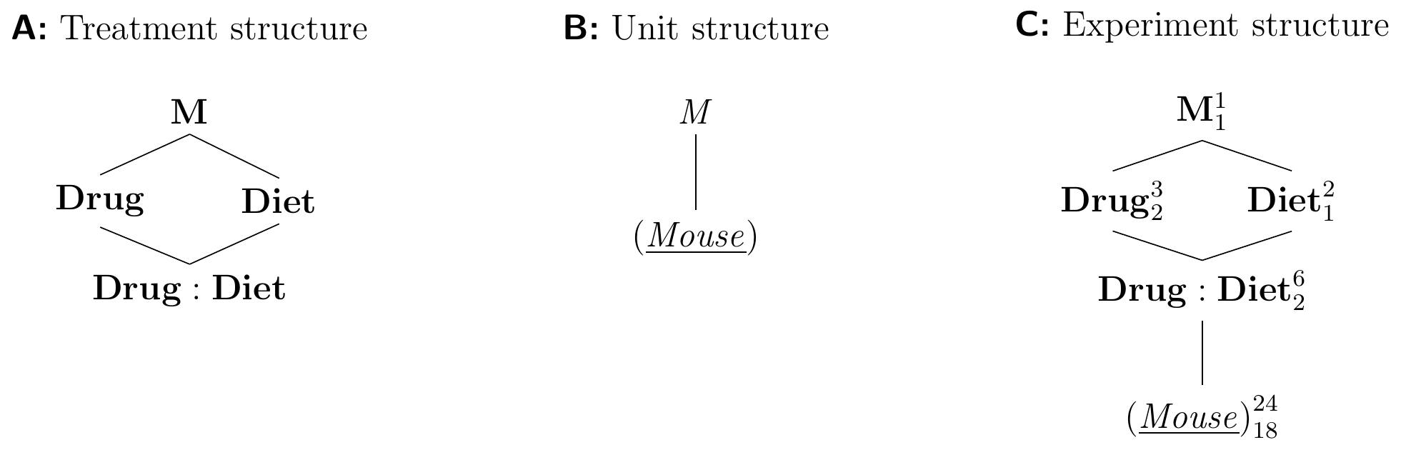
Figure 6.3: Completely randomized design for determining the effects of two different drugs and placebo combined with two different diets using four mice per combination of drug and diet, and a single response measurement per mouse.
6.3 ANOVA for Two Treatment Factors
The analysis of variance framework readily extends to more than one treatment factor. We already find all the new properties of this extension with only two factors, and we can therefore focus on this case for the moment.
6.3.1 Linear Model
For our general discussion, we consider two treatment factors A with \(a\) levels and B with \(b\) levels; the interaction factor A:B then has \(a\cdot b\) levels. We again denote by \(n\) the number of experimental units for each treatment combination in a balanced design, and by \(N=a\cdot b\cdot n\) the total sample size. For our example \(a=3\), \(b=2\), \(n=4\), and thus \(N=24\).
Cell Means Model
A simple linear model is the cell means model \[ y_{ijk} = \mu_{ij} + e_{ijk}\;, \] in which each cell mean \(\mu_{ij}\) is the average response of the experimental units receiving level \(i\) of the first treatment factor and level \(j\) of the second treatment factor and \(e_{ijk}\sim N(0,\sigma_e^2)\) is the residual of the \(k\)th replicate for the treatment combination \((i,j)\).
Our example leads to \(3\times 2=6\) cell means \(\mu_{11},\dots,\mu_{32}\); the cell mean \(\mu_{11}\) is the average response to the placebo treatment under the low fat diet, and \(\mu_{32}\) is the average response to the \(D2\) drug treatment under the high fat diet.
The cell means model does not explicitly reflect the factorial treatment design, and we could analyze our experiment as a one-way ANOVA with six treatment levels, as we did in the tumor diameter example in Section 5.4.
Parametric Model
The parametric model \[ y_{ijk} = \underbrace{\mu_{\bigcdot\bigcdot}}_{\mu} + \underbrace{(\mu_{i\bigcdot}-\mu_{\bigcdot\bigcdot})}_{\alpha_i} + \underbrace{(\mu_{\bigcdot j}-\mu_{\bigcdot\bigcdot})}_{\beta_j} + \underbrace{(\mu_{ij}-\mu_{i\bigcdot}-\mu_{\bigcdot j}+\mu_{\bigcdot\bigcdot})}_{(\alpha\beta)_{ij}} + e_{ijk}\;, \] makes the factorial treatment design explicit. Each cell mean \(\mu_{ij}\) is decomposed into four contributions: a grand mean \(\mu\), the average deviation of cell mean \(\mu_{i\bigcdot}\) for level \(i\) of A (averaged over all levels of B), the average deviation of cell mean \(\mu_{\bigcdot j}\) of B (averaged over all levels of A), and an interaction for each level of A:B.
The model components are shown schematically in Figure 6.4A for our drug-diet example. Each drug corresponds to a row, and \(\mu_{i\bigcdot}\) is the average response for drug \(i\), where the average is taken over both diets in row \(i\). Each diet corresponds to a column, and \(\mu_{\bigcdot j}\) is the average response for column \(j\) (over the three drugs). The interaction is the difference between the additive effect of the row and column differences to the grand mean \(\mu_{i\bigcdot}-\mu_{\bigcdot\bigcdot}\) and \(\mu_{\bigcdot j}-\mu_{\bigcdot\bigcdot}\), and the actual cell mean’s difference \(\mu_{ij}-\mu_{\bigcdot\bigcdot}\) from the grand mean: \[ \mu_{ij}-\mu_{i\bigcdot}-\mu_{\bigcdot j}+\mu_{\bigcdot\bigcdot} = (\mu_{ij}-\mu_{\bigcdot\bigcdot}) \,-\, \left((\mu_{i\bigcdot}-\mu_{\bigcdot\bigcdot}) \,+\, (\mu_{\bigcdot j}-\mu_{\bigcdot\bigcdot})\right)\;. \]
The model has five sets of parameters: \(a\) parameters \(\alpha_i\) and \(b\) parameters \(\beta_j\) constitute the main effect parameters of factor A and B, respectively, while the \(a\cdot b\) parameters \((\alpha\beta)_{ij}\) are the interaction effect parameters of factor A:B. They correspond to the factors in the experiment diagram: in our example, the factor M is associated by the grand mean \(\mu\), while the two treatment factors Drug and Diet are associated with \(\alpha_i\) and \(\beta_j\), respectively, and the interaction factor Drug:Diet with \((\alpha\beta)_{ij}\). The unit factor (Mouse) has 24 levels, each reflecting the deviation of a specific mouse, and is represented by the residuals \(e_{ijk}\) and their variance \(\sigma_e^2\). The degrees of freedom are the number of independent estimates for each set of parameters.
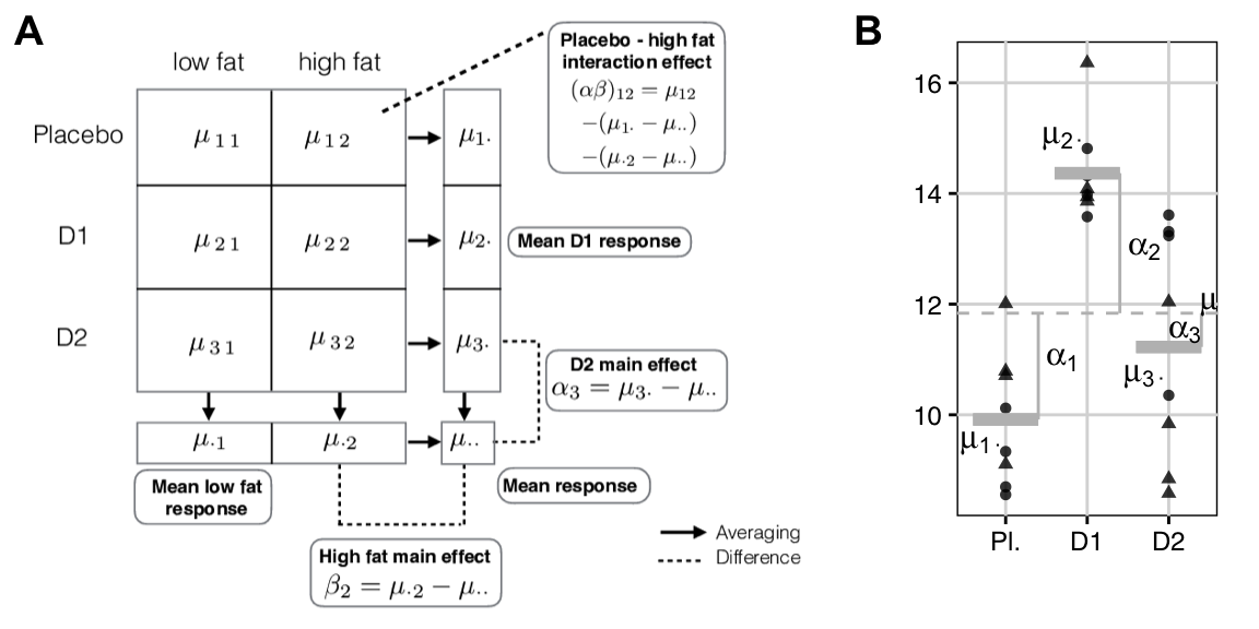
Figure 6.4: A: The 3-by-2 data table with averages per treatment. Main effects are differences between row- or column means and grand mean. Interaction effects are differences between cell means and the two main effects. B: Marginal data considered for drug pools data for each drug over diets. The three averages correspond to the row means and point shapes correspond to diet. Dashed line: grand mean; solid grey lines: group means; vertical lines: group mean deviations.
6.3.2 Analysis of Variance
The analysis of variance with more than one treatment factor is a direct extension of the one-way ANOVA, and is again based on decomposing sums of squares and degrees of freedom. Each treatment factor can be tested individually using a corresponding \(F\)-test.
Sums of Squares
For balanced designs, we decompose the sum of squares into one part for each factor in the design. The total sum of squares is \[ \text{SS}_\text{tot} = \text{SS}_\text{A} + \text{SS}_\text{B} + \text{SS}_\text{A:B} + \text{SS}_\text{res} = \sum_{i=1}^a\sum_{j=1}^b\sum_{k=1}^n(y_{ijk}-\bar{y}_{\bigcdot\bigcdot\bigcdot})^2\;, \] and measures the overall variation between the observed values and the grand mean. We now have two treatment sum of squares, one for factor A and one for B; they are the squared differences of the group mean from the grand mean: \[ \text{SS}_\text{A}\!\!=\!\!\sum_{i=1}^a\sum_{j=1}^b\sum_{k=1}^n(\bar{y}_{i\bigcdot\bigcdot}-\bar{y}_{\bigcdot\bigcdot\bigcdot})^2 \!=\! bn\sum_{i=1}^a(\bar{y}_{i\bigcdot\bigcdot}-\bar{y}_{\bigcdot\bigcdot\bigcdot})^2 \text{ and } \text{SS}_\text{B}\!=\!an\sum_{j=1}^b(\bar{y}_{\bigcdot j\bigcdot}-\bar{y}_{\bigcdot\bigcdot\bigcdot})^2\;. \] Each treatment sum of squares is found by pooling the data over all levels of the other treatment factor. For instance, \(\text{SS}_{\text{drug}}\) in our example results from pooling data over the diet treatment levels, corresponding to a one-way ANOVA situation as in Figure 6.4B.
The interaction sum of squares for A:B is \[ \text{SS}_\text{A:B} = n\sum_{i=1}^a\sum_{j=1}^b(\bar{y}_{ij\bigcdot}-\bar{y}_{i\bigcdot\bigcdot}-\bar{y}_{\bigcdot j\bigcdot}+\bar{y}_{\bigcdot\bigcdot\bigcdot})^2\;. \] If interactions exist, parts of \(\text{SS}_\text{tot}-\text{SS}_\text{A}-\text{SS}_\text{B}\) are due to a systematic difference between the additive prediction for each group mean, and the actual mean of that treatment combination.
The residual sum of squares measures the distances of responses to their corresponding treatment means: \[ \text{SS}_\text{res} = \sum_{i=1}^a\sum_{j=1}^b\sum_{k=1}^n(y_{ijk}-\bar{y}_{ij\bigcdot})^2\;. \] For our example, we find that \(\text{SS}_\text{tot}=\) 129.44 decomposes into treatments \(\text{SS}_\text{drug}=\) 83.73 and \(\text{SS}_\text{diet}=\) 0.59, interaction \(\text{SS}_\text{drug:diet}=\) 19.78 and residual \(\text{SS}_\text{res}=\) 25.34 sums of squares.
Degrees of Freedom
The degrees of freedom also partition by the corresponding factors, and the rules for Hasse diagrams allow quick and easy calculation. For the general two-way ANOVA, we have \[ \text{df}_\text{tot}\!=\!abn-1\!=\!\text{df}_\text{A} + \text{df}_\text{B} + \text{df}_\text{A:B} + \text{df}_\text{res}\!=\!(a-1) + (b-1) + (a-1)(b-1) + ab(n-1). \] With \(a=3\), \(b=2\), \(n=4\) for our example, we find \(\text{df}_\text{drug}=\) 2, \(\text{df}_\text{diet}=\) 1, \(\text{df}_\text{drug:diet}=\) 2, and \(\text{df}_\text{res}=\) 18, in correspondence with the Hasse diagram.
Mean Squares
Mean squares are found by dividing the sum of squares terms by their degrees of freedom. For example, we can calculate the total mean squares \[ \text{MS}_\text{tot} = \frac{\text{SS}_\text{tot}}{abn-1}\;, \] which corresponds to the variance in the data ignoring treatment groups. Further, \(\text{MS}_\text{A} = \text{SS}_\text{A}/ \text{df}_\text{A}\), \(\text{MS}_\text{B} = \text{SS}_\text{B} / \text{df}_\text{B}\), \(\text{MS}_\text{A:B} = \text{SS}_\text{A:B} / \text{df}_\text{A:B}\), and \(\text{MS}_\text{res} = \text{SS}_\text{res} / \text{df}_\text{res}\). In our example, \(\text{MS}_\text{drug}=\) 41.87, \(\text{MS}_\text{diet}=\) 0.59, \(\text{MS}_\text{drug:diet}=\) 9.89, and \(\text{MS}_\text{res}=\) 1.41.
\(F\)-tests
We can perform an omnibus \(F\)-test for each factor by comparing its mean squares with the corresponding residual mean squares. We find the correct denominator mean squares from the experiment structure diagram: it corresponds to the closest random factor below the tested treatment factor and is \(\text{MS}_\text{res}\) from (Mouse) for all three tests in our example.
The two main effect tests for and based on the \(F\)-statistics \[ F = \frac{\text{MS}_\text{A}}{\text{MS}_\text{res}}\sim F_{a-1,ab(n-1)} \quad\text{and}\quad F = \frac{\text{MS}_\text{B}}{\text{MS}_\text{res}} \sim F_{b-1,ab(n-1)} \] test the two hypotheses \[ H_{0,\mathbf{A}}: \mu_{1\bigcdot}=\cdots=\mu_{a\bigcdot} \quad\text{and}\quad H_{0,\mathbf{B}}: \mu_{\bigcdot 1}=\cdots=\mu_{\bigcdot b}\;, \] respectively. These hypotheses state that the corresponding treatment groups, averaged over the levels of the other factor, have equal means and the average effect of the corresponding factor is zero. The treatment mean squares have expectations \[ \mathbb{E}(\text{MS}_\text{A}) = \sigma_e^2 + \frac{nb}{a-1}\sum_{i=1}^a\alpha_i^2 \quad\text{and}\quad \mathbb{E}(\text{MS}_\text{B}) = \sigma_e^2 + \frac{na}{b-1}\sum_{j=1}^b\beta_j^2\;, \] which both provide an independent estimate of the residual variance \(\sigma_e^2\) if the corresponding null hypothesis is true.
The interaction test for is based on the \(F\)-statistic \[ F = \frac{\text{MS}_\text{A:B}}{\text{MS}_\text{res}}\sim F_{(a-1)(b-1),ab(n-1)}\;, \] and the mean squares term has expectation \[ \mathbb{E}(\text{MS}_\text{A:B}) = \sigma_e^2 + \frac{n}{(a-1)(b-1)} \sum_{i=1}^a\sum_{j=1}^b (\alpha\beta)_{ij}^2\;. \] Thus, the corresponding null hypothesis is \(H_{0, \mathbf{A:B}}: (\alpha\beta)_{ij}=0\) for all \(i,j\). This is equivalent to \[ H_{0, \mathbf{A:B}}: \mu_{ij} = \mu + \alpha_i + \beta_j \text{ for all } i,j\;, \] stating that each treatment group mean has a contribution from both factors, and these contributions are independent of each other.
ANOVA Table
Using R, these calculations are done easily using aov(). We find the model specification from the Hasse diagrams. All fixed factors are in the treatment structure and provide the terms 1+drug+diet+drug:diet which we abbreviate as drug*diet. All random factors are in the unit structure, providing Error(mouse), which we may drop from the specification since (Mouse) is the lowest random unit factor. The model y~drug*diet yields the ANOVA table
| Df | Sum Sq | Mean Sq | F value | Pr(>F) | |
|---|---|---|---|---|---|
| drug | 2 | 83.73 | 41.87 | 29.74 | 1.97e-06 |
| diet | 1 | 0.59 | 0.59 | 0.42 | 5.26e-01 |
| drug:diet | 2 | 19.78 | 9.89 | 7.02 | 5.56e-03 |
| Residuals | 18 | 25.34 | 1.41 |
We find that the sums of squares for the drug effect are large compared to all other contributors and Drug is highly significant. The Diet main effect does not achieve significance at any reasonable level, and its sums of squares are tiny. However, we find a large and significant Drug:Diet interaction and must therefore be very careful in our interpretation of the results, as we discuss next.
6.3.3 Interpretation of Main Effects
The main effect of a treatment factor is the deviation between group means of its factor levels, averaged over the levels of all other treatment factors.
In our example, the null hypothesis of the drug main effect is \[ H_{0,\text{drug}}:\;\mu_{1\bigcdot}=\mu_{2\bigcdot}=\mu_{3\bigcdot} \;\;\text{or equiv.}\;\; H_{0,\text{drug}}:\;\alpha_1=\alpha_2=\alpha_3=0\;, \] and the corresponding hypothesis for the diet main effect is \[ H_{0,\text{diet}}:\;\mu_{\bigcdot 1}=\mu_{\bigcdot 2} \;\;\text{or equiv.}\;\; H_{0,\text{diet}}:\;\beta_1=\beta_2=0\;, \] The first hypothesis asks if there is a difference in the enzyme levels between the three drugs, ignoring the diet treatment by averaging the observations for low fat and high fat diet for each drug. The second hypothesis asks if there is a difference between enzyme levels for the two diets, averaged over the three drugs.
From the ANOVA table, we see that the main effect of the drug treatment is highly significant, indicating that regardless of the diet, the drugs affect enzyme levels differently. In contrast, the diet main effect is negligibly small with a large \(p\)-value, but the raw data in Figure 6.2A show that while the diet has no influence on the drug levels when averaged over all drug treatments, it has visible effects for some drugs: the effect of \(D1\) seems to be unaffected by the diet, while a low fat diet yields higher enzyme levels for \(D2\), but lower levels for placebo.
6.3.4 Interpretation of Interactions
The interaction effects quantify how different the effect of one factor is for different levels of another factor. For our example, the large and significant interaction factor shows that while the diet main effect is negligible, the two diets have very different effect depending on the drug treatment. Simply because the diet main effect is not significant therefore does not mean that the diet effect can be neglected for each drug. The most important rule when analyzing designs with factorial treatment structures is therefore:
Be careful when interpreting main effects in the presence of large interactions.
Four illustrative examples of interactions are shown in Figure 6.5 for two factors A and B with two levels each. In each panel, the two levels of A are shown on the horizontal axis, and a response on the vertical axis. The two lines connect the same levels of factor B between levels of A.
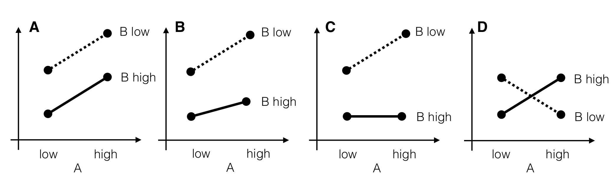
Figure 6.5: Four stylized scenarios with different interactions. A: Parallel lines indicate no interaction and an additive model. B: Small interaction and nonzero main effects. Factor B attenuates effect of factor A. C: Strongly pronounced interaction. Factor B on high level completely compensates effect of factor A. D: Complete effect reversal; all information on factor effects is in the interaction.
In the first case (Fig. 6.5A), the two lines are parallel and the difference in response between the low to the high levels of B is the same for both levels of A, and vice-versa. The average responses \(\mu_{ij}\) in each of the four treatment groups are then fully described by an additive model \[ \mu_{ij} = \mu + \alpha_i + \beta_j\;, \] with no interaction and \((\alpha\beta)_{ij}=0\).
In our example, we might compare the responses to placebo and drug \(D1\) between diets with almost parallel lines in Figure 6.2B. The two cell means \(\mu_{11}\) for placebo and \(\mu_{21}\) for \(D1\) under a low fat diet are \[ \mu_{11} = \mu+\alpha_1+\beta_1 \quad\text{and}\quad \mu_{21} = \mu+\alpha_2+\beta_1\;, \] with difference \(\mu_{21}-\mu_{11}=\alpha_2-\alpha_1\). Under a high fat diet, the cell means are \[ \mu_{12} = \mu+\alpha_1+\beta_2 \quad\text{and}\quad \mu_{22} = \mu+\alpha_2+\beta_2 \;, \] and their difference is also \(\mu_{22}-\mu_{12}=\alpha_2-\alpha_1\).
In other words, the difference between the two drugs is independent of the diet and conversely the difference between the two diets is independent of the drug administered. We can then interpret the drug effect without regard for the diet and speak of a “drug effect” or conversely interpret the diet effect independently of the drug and speak of a “diet effect.”
It might also be that the true situation for placebo and \(D1\) is more similar to Figure 6.5B, a quantitative interaction: the increase in response from high to low level for factor B is more pronounced if A is on the high level, yet we achieve higher responses for B low under any level of A, and conversely a higher response is achieved by using A on the high level for both levels of B. Then, the effects of treatments A and B are not simply additive, and the interaction term \[ (\alpha\beta)_{ij} = \mu_{ij} - (\mu+\alpha_i+\beta_j) \] quantifies exactly how much the observed cell mean \(\mu_{ij}\) differs from the value predicted by the additive model \(\mu+\alpha_i+\beta_j\).
For our example, the responses to placebo and drug \(D1\) under a low fat diet are then \[ \mu_{11} = \mu+\alpha_1+\beta_1+(\alpha\beta)_{11} \quad\text{and}\quad \mu_{21} = \mu+\alpha_2+\beta_1 +(\alpha\beta)_{21}\;, \] and thus the difference is \(\mu_{21}-\mu_{11}=(\alpha_2-\alpha_1)+((\alpha\beta)_{21}-(\alpha\beta)_{11})\), while for the high fat diet, we find a difference between placebo and \(D1\) of \(\mu_{22}-\mu_{12}=(\alpha_2-\alpha_1)+((\alpha\beta)_{22}-(\alpha\beta)_{12})\). If at least one of the parameters \((\alpha\beta)_{ij}\) is not zero, then the difference between \(D1\) and placebo depends on the diet. The interaction is the difference of differences \[ \underbrace{(\mu_{21}-\mu_{11})}_{\text{low fat}} - \underbrace{(\mu_{22}-\mu_{12})}_{\text{high fat}} = \left(\,(\alpha\beta)_{21}-(\alpha\beta)_{11}\,\right) - \left(\,(\alpha\beta)_{22}-(\alpha\beta)_{12}\,\right)\;, \] and is fully described by the four interaction parameters corresponding to the four means involved.
It is then misleading to speak of a “drug effect,” since this effect is diet-dependent. In our case of a quantitative interaction, we find that a placebo treatment always gives lower enzyme levels, independent of the diet. The diet only modulates this effect, and we can achieve a greater increase in enzyme levels for \(D1\) over placebo if we additionally use a low fat diet.
The interaction becomes more pronounced the more “non-parallel” the lines become. The interaction in Figure 6.5C is still quantitative and a low level of B always yields the higher response, but the modulation by A is much stronger than before. In particular, A has no effect under a high level of B and using either a low or high level yields the same average response, while under a low level of B, using a high level for A yields even higher responses.
In our example, there is an additional quantitative interaction between diet and \(D1\)/\(D2\), with \(D1\) consistently giving higher enzyme levels than \(D2\) under both diets. However, if we would only consider a low fat diet, then the small difference between responses to \(D1\) and \(D2\) might make us prefer \(D2\) if it is much cheaper or has a better safety profile, for example, while \(D2\) is no option under a high fat diet.
Interactions can also be qualitative, in which case we might see an effect reversal. Now, one level of B is no longer universally superior under all levels of A, as shown in Figure 6.5D for an extreme case. If A is on the low level, then higher responses are gained if B is on the low level, while for A on its high level, the high level of B gives higher responses.
We find this situation in our example when comparing the placebo treatment and \(D2\): under a low fat diet, \(D2\) shows higher enzyme levels, while enzyme levels are similar or even lower for \(D2\) than placebo under a high fat diet. In other words, \(D1\) is always superior to a placebo and we can universally recommend its use, but we should only use \(D2\) for a low fat diet since it seems to have little to no (or even negative) effect under a high fat diet.
6.3.5 Effect Sizes
We measure the effect size of each factor using its \(f^2\) value. For our generic two-factor design with factors A and B with \(a\) and \(b\) levels, respectively, the effect sizes are \[ f^2_\text{A} = \frac{1}{a\sigma_e^2}\sum_{i=1}^a \alpha_i^2 \,, \quad f^2_\text{B} = \frac{1}{b\sigma_e^2}\sum_{j=1}^b \beta_j^2 \,, \quad f^2_\text{A:B} = \frac{1}{ab\sigma_e^2}\sum_{i=1}^a\sum_{j=1}^b (\alpha\beta)_{ij}^2 \,, \] which in our example are \(f^2_\text{drug}=\) 0.43 (huge), \(f^2_\text{diet}=\) 0.02 (tiny), and \(f^2_\text{drug:diet}=\) 0.3 (medium).
Alternatively, we can measure the effect of factor X by its variance explained \(\eta^2_\text{X}=\text{SS}_\text{X}/\text{SS}_\text{tot}\), which in our example yields \(\eta^2_\text{drug}=\text{SS}_\text{drug}/\text{SS}_\text{tot} =\) 65% for the drug main effect, \(\eta^2_\text{diet}=\) 0.45% for the diet main effect, and \(\eta^2_\text{drug:diet}=\) 15% for the interaction. This effect size measure has two caveats for multi-way ANOVAs, however. First, the total sum of squares contains all those parts of the variation ‘explained’ by the other treatment factors. The magnitude of any \(\eta^2_\text{X}\) therefore depends on the number of other treatment factors, and on the proportion of variation explained by them. The second caveat is a consequence of this: the explained variance \(\eta^2_{X}\) does not have a simple relationship with the effect size \(f^2_{X}\), which compares the variation due to the factor alone to the residual variance and excludes all effects due to other treatment factors.
We resolve both issues by the partial-\(\eta^2\) effect size measure, which is the fraction of variation explained by each factor over the variation that remains to be explained after accounting for all other treatment factors: \[ \eta^2_\text{p, A} = \frac{\text{SS}_\text{A}}{\text{SS}_\text{A}+\text{SS}_\text{res}}\,, \quad \eta^2_\text{p, B} = \frac{\text{SS}_\text{B}}{\text{SS}_\text{B}+\text{SS}_\text{res}}\,, \quad \eta^2_\text{p, A:B} = \frac{\text{SS}_\text{A:B}}{\text{SS}_\text{A:B}+\text{SS}_\text{res}}\,. \] Note that \(\eta_\text{p, X}^2=\eta_\text{X}^2\) for a one-way ANOVA. The partial-\(\eta^2\) are not a partition of the variation into single factor contributions and therefore do not sum to one, but they have a direct relation to \(f^2\): \[ f^2_\text{X} = \frac{\eta^2_\text{p, X}}{1-\eta^2_\text{p, X}} \] for any treatment factor X. In our example, we find \(\eta^2_\text{p, drug}=\) 77%, \(\eta^2_\text{p, diet}=\) 2%, and \(\eta^2_\text{p, drug:diet}=\) 44%.
6.3.6 Model Reduction and Marginality Principle
In the one-way ANOVA, the omnibus \(F\)-test was of limited use for addressing our scientific questions. With more factors in the experiment design, however, a non-significant \(F\)-test and a small effect size would allow us to remove the corresponding factor from the model. This is known as model reduction, and the reduced model is often easier to analyze and to interpret.
In order to arrive at an interpretable reduced model, we need to take account of the principle of marginality for model reduction (Nelder 1994):
If we remove a factor from the model, then we also need to remove all interaction factors involving this factor.
For a two-way ANOVA, the marginality principle implies that only the interaction factor can be removed in the first step. We then re-estimate the resulting additive model and might further remove one or both main effects factors if their effects are small and non-significant. If the interaction factor cannot be removed, then the two-way ANOVA model cannot be reduced.
Indeed, the interpretation of the model would suffer severely if we removed A but kept A:B, and this model would then describe B as nested in A, in contrast to the actual design which has A and B crossed. The resulting model is then of the form
\[
y_{ijk} = \mu + \alpha_i + (\alpha\beta)_{ij} + e_{ijk}
\]
and has three sets of parameters: the grand mean, one deviation for each level of A, and additionally different and independent deviations for the levels of B within each level of A. We see this consequence of violating the marginality principle by comparing the full model diagram in Figure 6.6A to the diagram of the reduced model in Figure 6.6B and recalling that two nested factors correspond to a main effect and an interaction effect since A/B=A+A:B.
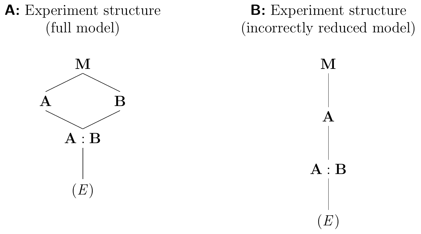
Figure 6.6: A: Experiment structure diagram for full two-way model with interaction. Factors A and B are crossed. B: Experiment structure resulting from removing one treatment factor but not its interaction, violating the marginality principle. Factor B is now nested in A contrary to actual design.
In our example, we find that Diet has a non-significant \(p\)-value and small effect size, which suggests that it does not have an appreciable main effect when averaged over drugs. However, Diet is involved in the significant interaction factor Drug:Diet with large effect size, and the marginality principle prohibits removing Diet from the model. Indeed, we have seen that the diet has an appreciable effect on how the three drugs compare, and modifies and even reverses their effects, so we cannot ignore it.
6.3.7 Estimated Marginal Means
Recall that the estimated marginal means give the average response in a treatment group calculated from a linear model. To solidify our understanding of estimated marginal means, we briefly consider their calculation and interpretation for our example. This also further exemplifies the interpretation of interactions and the consequences of model reduction.
Our example has six possible cell means, one for each combination of a drug with a diet. We consider five linear models for this factorial design with two crossed treatment factors: the full model with interaction, the additive model, two models with a single treatment factor, and a model with no treatment factors. Each of these models gives rise to different estimated marginal means for the six treatment combinations, and their predicted cell means are shown in Table 6.2.
| Drug | Diet | Data | Full | Additive | Drug only | Diet only | Average |
|---|---|---|---|---|---|---|---|
| Placebo | low fat | 9.18 | 9.18 | 10.07 | 9.92 | 11.99 | 11.84 |
| D1 | low fat | 14.17 | 14.17 | 14.52 | 14.37 | 11.99 | 11.84 |
| D2 | low fat | 12.63 | 12.63 | 11.38 | 11.23 | 11.99 | 11.84 |
| Placebo | high fat | 10.65 | 10.65 | 9.76 | 9.92 | 11.68 | 11.84 |
| D1 | high fat | 14.56 | 14.56 | 14.21 | 14.37 | 11.68 | 11.84 |
| D2 | high fat | 9.83 | 9.83 | 11.07 | 11.23 | 11.68 | 11.84 |
The Full model is \(\mu_{ij} = \mu + \alpha_i + \beta_j + (\alpha\beta)_{ij}\) and has specification y~1+drug+diet+drug:diet. It provides six different and independent cell means, which are identical to the empirical averages (Data) for each cell.
The Additive model is \(\mu_{ij}=\mu+\alpha_i+\beta_j\) and is specified by y~1+drug+diet. It does not have an interaction term and the two treatment effects are hence additive, such that the difference between \(D1\) and placebo, for example, is \(10.07-14.52=-4.45\) for a low fat diet and \(9.76-14.21=-4.45\) for a high fat diet. In other words, differences between drugs are independent of the diet and vice-versa.
The two models Drug only and Diet only are \(\mu_{ij}=\mu+\alpha_i\) (specified as y~1+drug) and \(\mu_{ij}=\mu+\beta_j\) (specified as y~1+diet) and completely ignore the respective other treatment. The first gives identical estimated marginal means for all conditions under the same drug and thus predicts three different cell means, while the second gives identical estimated marginal means for all conditions under the same diet, predicting two different cell means. Finally, the Average model \(\mu_{ij}=\mu\) is specified as y~1 and describes the data by a single common mean, resulting in identical predictions for the six cell means.
Hence, the model used for describing the experimental data determines the estimated marginal means, and therefore the contrast estimates. In particular, nonsense will arise if we use an additive model such as drug+diet for defining the estimated marginal means, and then try to estimate an interaction contrast (cf. Section 6.6.2) using these means. The contrast is necessarily zero, and no standard error or \(t\)-statistic can be calculated.
6.3.8 A Real-Life Example—Drug Metabolization Continued
In Section 5.4, we looked into a real-life example and examined the effect of two anticancer drugs (IFF and CP) and an inhibitor (RTV) on tumor growth. We analyzed the data using a one-way ANOVA based on six treatment groups and concentrated on relevant contrasts. There is, however, more structure in the treatment design, since we are actually looking at combinations of an anticancer drug and an inhibitor. To account for this structure, we reformulate the analysis to a more natural two-way ANOVA with two treatment factors: Drug with the three levels none, CP, and IFF, and Inhibitor with two levels none and RTV. Each drug is used with and without inhibitor, leading to a fully-crossed factorial treatment design with the two factors and their interaction Drug:Inhibitor. We already used the two conditions (none,none) and (none,RTV) as our control conditions in the contrast analysis. The model specification is Diameter~Drug*Inhibitor and leads to the ANOVA table
| Df | Sum Sq | Mean Sq | F value | Pr(>F) | |
|---|---|---|---|---|---|
| Drug | 2 | 495985.17 | 247992.58 | 235.05 | 4.11e-29 |
| Inhibitor | 1 | 238533.61 | 238533.61 | 226.09 | 5.13e-22 |
| Drug:Inhibitor | 2 | 80686.12 | 40343.06 | 38.24 | 1.96e-11 |
| Residuals | 60 | 63303.4 | 1055.06 |
We note that the previous sum of squares for Condition was 815204.90 in our one-way analysis and now exactly partitions into the contributions of our three treatment factors. The previous effect size of 93% is also partitioned into \(\eta^2_{\text{Drug}}=\) 56%, \(\eta^2_{\text{Inhibitor}}=\) 27%, and \(\eta^2_{\text{Drug:Inhibitor}}=\) 9%. In other words, the differences between conditions are largely caused by differences between the anticancer drugs, but the presence of the inhibitor also explains more than one-quarter of the variation. The interaction is highly significant and cannot be ignored, but its effect is much smaller compared to the two main effects. All of this is of course in complete agreement with our previous contrast analysis.
6.4 More on Factorial Designs
We briefly discuss the general advantages of factorial treatment designs and extend our discussion to more than two treatment factors.
6.4.1 Advantage of Factorial Treatment Design
Before the advantages of simultaneously using multiple crossed treatment factors in a factorial designs were fully understood by practitioners, so-called one variable at a time (OVAT) designs were commonly used for studying the effect of multiple treatment factors. Here, only a single treatment factor was considered in each experiment, while all other treatment factors were kept at a fixed level to achieve maximally controlled conditions for studying each factor. These designs do not allow estimation of interactions and can therefore lead to incorrect interpretation if interactions are present. In contrast, factorial designs reveal interaction effects if they are present and provide the basis for correct interpretation of the experimental effects. The mistaken logic of OVAT designs was clearly recognized by R. A. Fisher in the 1920s:
No aphorism is more frequently repeated in connection with field trials, than that we must ask Nature few questions, or, ideally, one question, at a time. The writer is convinced that this view is wholly mistaken. Nature, he suggests, will best respond to a logical and carefully thought out questionnaire; indeed, if we ask her a single question, she will often refuse to answer until some other topic has been discussed. (Fisher 1926)
Slightly less obvious is the fact that factorial designs also require smaller sample sizes than OVAT designs, even if no interactions are present between the treatment factors. For example, we can estimate the main effects of two factors A and B with two levels each using two OVAT designs with \(2n\) experimental units per experiment. Each main effect is then estimated with \(2n-2\) residual degrees of freedom. We can use the same experimental resources for a \(2\times 2\)-factorial design with \(4n\) experimental units. If the interaction A:B is large, then only this factorial design will allow correct inferences. If the interaction is negligible, then we have two estimates of the A main effect: first for B on the low level by contrasting the \(n\) observations for A on a low level with those \(n\) for A on a high level, and second for the \(n+n\) observations for B on a high level. The A main effect estimate is then the average of these two, based on all \(4n\) observations; this is sometimes called hidden replication. The inference on A is also more general, since we observe the A effect under two conditions for B. The same argument holds for estimating the B main effect. Since we need to estimate one grand mean and one independent group mean each for A and B, the residual degrees of freedom are \(4n-3\).
6.4.2 One Observation per Cell
Constraints on resources or complicated logistics for the experiment sometimes do not permit replication within each experimental condition, and we then have a single observation for each treatment combination. The Hasse diagram in Figure 6.7A shows the resulting experiment structure for two generic factors A and B with \(a\) and \(b\) levels, respectively, and one observation per combination. We do not have degrees of freedom for estimating the residual variance, and we can neither estimate confidence intervals for establishing the precision of estimates nor perform hypothesis tests. If large interactions are suspected, then this design is fundamentally flawed.
Removing Interactions
The experiment can be successfully analyzed using an additive model \(\mu_{ij}=\mu+\alpha_i+\beta_j\) if interactions are small enough to be ignored, such that \((\alpha\beta)_{ij}\approx 0\). We can then remove the interaction factor from the full model, which leads to new residuals \((\alpha\beta)_{ij}+e_{ij}\approx e_{ij}\) and ‘frees up’ \((a-1)(b-1)\) degrees of freedom for estimating their residual variance. This strategy corresponds to merging the A:B interaction factor with the experimental unit factor (E), resulting in the experimental structure in Figure 6.7B.
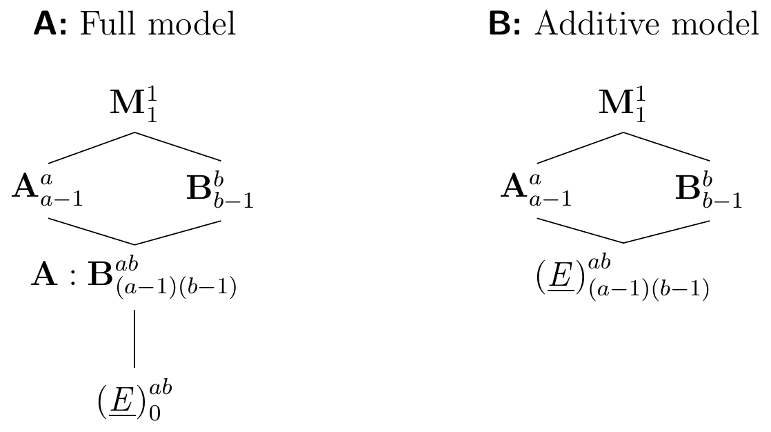
Figure 6.7: A: Experiment structure for \(a\times b\) two-way factorial with single observation per cell; no residual degrees of freedom left. B: Same experiment based on additive model removes interaction factor and frees degrees of freedom for estimating residual variance.
Tukey’s Method for Testing Interactions
The crucial assumption of no interaction is sometimes justified on subject-matter grounds or from previous experience. If a non-replicated factorial design is run without a clear justification, we can use an ingenious procedure by Tukey to test for an interaction (Tukey 1949b). It applies if at least one of the two treatment factors has three levels or more. Instead of the full model with interaction, Tukey proposed to use a more restricted version of the interaction: a multiple of the product of the two main effects. The corresponding model is \[ y_{ij} = \mu + \alpha_i + \beta_j + \tau\cdot\alpha_i\cdot\beta_j + e_{ij}\;, \] an additive model based solely on the main effect parameters, augmented by a special interaction term that introduces a single additional parameter \(\tau\) and requires only one rather than \((a-1)(b-1)\) degrees of freedom. If the hypothesis \(H_0: \tau=0\) of no interaction is true, then the test statistic \[ F = \frac{\text{SS}_\tau /1 }{\text{MS}_\text{res}} \sim F_{1,ab-(a+b)} \] has an \(F\)-distribution with one numerator and \(ab-(a+b)\) denominator degrees of freedom.
Here, the ‘interaction’ sum of squares is calculated as \[ \text{SS}_\tau = \frac{\left(\sum_{i=1}^a\sum_{j=1}^b y_{ij}\cdot(\bar{y}_{i\bigcdot}-\bar{y}_{\bigcdot\bigcdot}) \cdot (\bar{y}_{\bigcdot j}-\bar{y}_{\bigcdot\bigcdot})\right)^2} {\Big(\sum_{i=1}^a(\bar{y}_{i\bigcdot}-\bar{y}_{\bigcdot\bigcdot})^2\Big) \cdot \Big(\sum_{j=1}^b(\bar{y}_{\bigcdot j}-\bar{y}_{\bigcdot\bigcdot})^2\Big)}\;. \] and has one degree of freedom.
Lenth’s Method for Analyzing Unreplicated Factorials
An alternative method for analyzing a non-replicated factorial design was proposed in Lenth (1989). It crucially depends on the assumption that most effects are small and negligible, and only a fraction of all effects is active and therefore relevant for the analysis and interpretation.
The main idea is then to calculate a robust estimate of the standard error based on the assumption that most deviations are random and not caused by treatment effects. This error estimate is then used to discard factors whose effects are sufficiently small to be negligible.
Specifically, we denote the estimated average difference between low and high level of the \(j\)th factor by \(c_j\) and estimate the standard error as 1.5 times the median of absolute effect estimates: \[ s_0 = 1.5 \cdot \text{median}_{j} |c_j|\;. \] If no effect were active, then \(s_0\) would already provide an approximate estimate of the standard error. If some effects are active, they inflate the estimate by an unknown amount. We therefore restrict our estimation to those effects that are ‘small enough’ and do not exceed 2.5 times the current standard error estimate. The pseudo standard error is then \[ \text{PSE} = 1.5 \cdot \text{median}_{|c_j|<2.5\cdot s_0} |c_j|\;. \] The margin of error (ME) (an upper limit of a confidence interval) is then \[ \text{ME} = t_{0.975, d} \cdot \text{PSE}\;, \] and Lenth proposes to use \(d=m/3\) as the degrees of freedom, where \(m\) is the number of effects in the model. This limit is corrected for multiple comparisons by adjusting the confidence limit from \(\alpha=0.975\) to \(\gamma=(1+0.95^{1/m})/2\). The resulting simultaneous margin of error (SME) is then \[ \text{SME} = t_{\gamma, d} \cdot \text{PSE}\;. \] Factors with effects exceeding SME in either direction are considered active, those between the ME limits are inactive, and those between ME and SME have unclear status. We therefore choose those factors that exceed SME as our safe choice, and might include those exceeding ME as well for subsequent experimentation.
In his paper, Lenth discusses a \(2^4\)-factorial experiment, where the effect of acid strength (S), time (t), amount of acid (A), and temperature (T) on the yield of isatin is studied (Davies 1954). The experiment design and the resulting yield are shown in Table 6.3.
|
|
The results are shown in Figure 6.8. No factor seems to be active, with temperature, acid strength, and the interaction of temperature and time coming closest. Note that the marginality principle requires that if we keep the temperature-by-time interaction, we must also keep the two main effects temperature and time in the model, regardless of their size or significance.
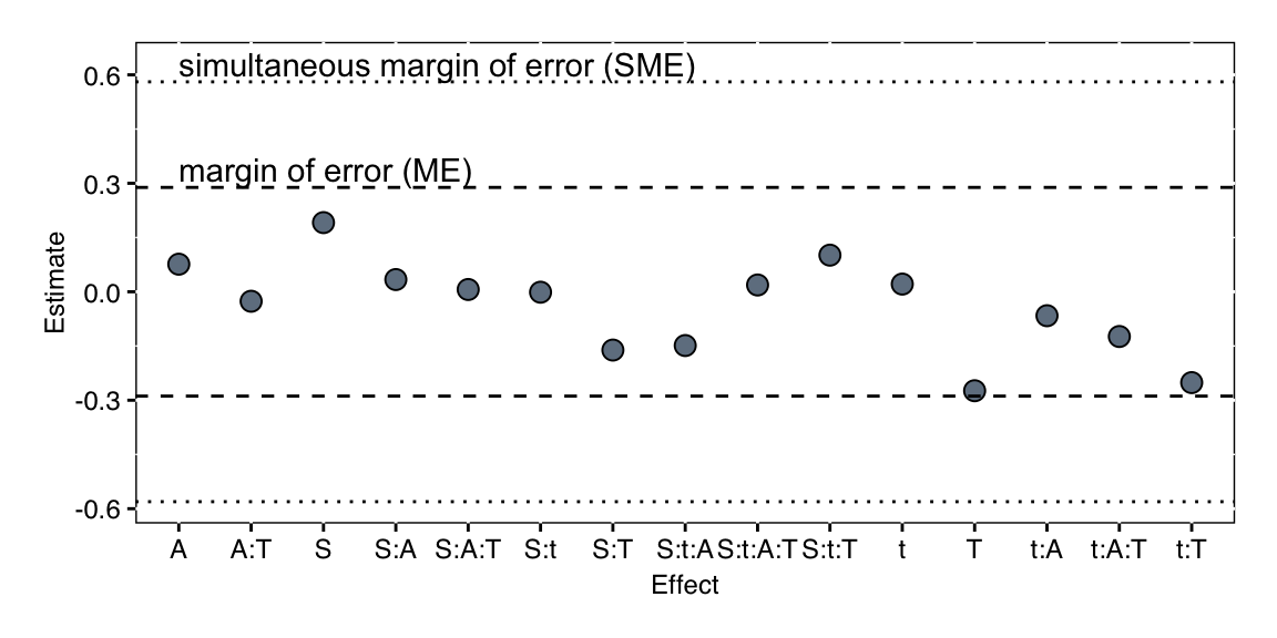
Figure 6.8: Analysis of active effects in unreplicated \(2^4\)-factorial with Lenth’s method.
6.4.3 Higher-Order Factorials
We can construct factorial designs for any number of factors with any number of levels, but the number of treatment combinations increases exponentially with the number of factors, and the more levels we consider per factor, the more combinations we get. For example, introducing the vendor as a third factor with two levels into our drug-diet example already yields \(3\cdot 2\cdot 2=12\) combinations, and introducing a fourth three-level factor increases this number further to \(12\cdot 3=36\) combinations. In addition, both extensions yield higher-order interactions between three and four factors.
A Model with Three Treatment Factors
We illustrate higher-order factorials using a three-way factorial with three treatment factors Drug with three levels, Diet (two levels), and Vendor (two levels). The experiment design is shown in Figure 6.9A with two replicates per treatment. The corresponding linear model is \[ y_{ijkl} = \mu_{ijk} + e_{ijkl} = \mu + \alpha_i + \beta_j + \gamma_k + (\alpha\beta)_{ij} + (\alpha\gamma)_{ik} + (\beta\gamma)_{jk} + (\alpha\beta\gamma)_{ijk} + e_{ijkl}\;. \] This model has three main effects, three two-way interactions and one three-way interaction. A large and significant three-way interaction \((\alpha\beta\gamma)_{ijk}\) arises, for example, if the drug-diet interaction that we observed for \(D2\) compared to placebo under both diets only occurs for the kit of vendor A, but not for the kit of vendor B (or with different magnitude). In other words, the two-way interaction itself depends on the level of the third factor and we are now dealing with a difference of a difference of differences.
In this particular example, we might consider reducing the model by removing all interactions involving Vendor, as there seems no plausible reason why the kit used for preparing the samples should interact with drug or diet. The resulting diagram is Figure 6.9B; this model reduction adheres to the marginality principle.
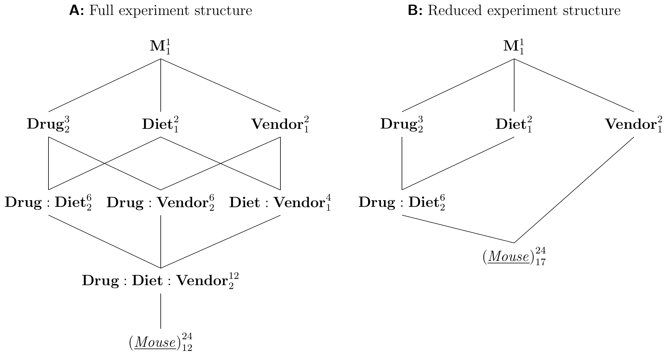
Figure 6.9: Three-way factorial. A: Full experiment structure with three two-way and one three-way interaction. B: Reduced experiment structure assuming negligible interactions with vendor.
A further example of a three-way analysis of variance inspired by an actual experiment concerns the inflammation reaction in mice and potential drug targets to suppress inflammation. It was already known that a particular pathway gets activated to trigger an inflammation response, and the receptor of that pathway is a known drug target. In addition, there was preliminary evidence that inflammation sometimes triggers even if the pathway is knocked out. A \(2\times 2\times 2=2^3\)-factorial experiment was conducted with three treatment factors: (i) genotype: wildtype mice / knock-out mice without the known receptor; (ii) drug: placebo treatment / known drug; (iii) waiting time: 5 hours / 8 hours between inducing inflammation and administering the drug or placebo. Several mice were used for each of the 8 combinations and their protein levels measured using mass spectrometry. The main focus of inference is the genotype-by-drug interaction, which would indicate if an alternate activation exists and how strong it is. The three-way interaction then provides additional information about difference in activation times between the known and a potential unknown pathway. We discuss this example in more detail in Section 9.8.6.
Strategies for High-order Factorials
The implementation and analysis of factorial designs becomes more challenging as the number of factors and their levels increases. First, the number of parameters and degrees of freedom increase rapidly with the order of the interaction. For example, if three treatment factors are considered with three levels each, then \(a=b=c=3\), yielding one grand mean parameter, \(a-1=b-1=c-1=2\) main effect parameters per factor (6 in total), \((a-1)(b-1)=4\) two-way interaction parameters per interaction (12 in total), and \((a-1)(b-1)(c-1)=8\) parameters for the three-way interaction, with a total of \(1+6+12+8=27\) parameters to describe the full model. Of course, this number is identical to the number \(3^3=27\) of possible treatment combinations (the model is saturated) and the experiment already requires 54 experimental units for two replicates.
In addition, the interpretation of an interaction becomes more intricate the higher its order: already a three-way interaction describes a difference of a difference of differences. In practice, interactions of order higher than three are rarely considered in a final model due to difficulties in interpretation, and already three-way interactions are not very common.
If significant higher-order interactions occur with considerable effect sizes, we can try to stratify the analysis by the one or several factors and provide separate analyses for each of the levels. For our example, with a significant and large three-way interaction, we could stratify by vendor and produce two separate models, one for vendor A and one for vendor B, studying the effect of drug and diet independently for both kits. The advantage of this approach is the easier interpretation, but we are also effectively halving the experiment size, such that information on drug and diet gained from one vendor does not transfer easily into information for the other vendor.
With more than three factors, even higher-order interactions can be considered. Statistical folklore and practical experience suggest that interactions often become less pronounced the higher their order, a heuristic known as effect sparsity. Thus, if there are no substantial two-way interactions, we do not expect relevant interactions of order three or higher.
If we have several replicate observations per treatment, then we can estimate the full model with all interactions and use the marginality principle to reduce the model by removing higher-order interactions that are small and non-significant. If only one observation per treatment group is available, a reasonable strategy is to remove the highest-order interaction term from the model in order to free its degrees of freedom. These are then used for estimating the residual variance, which in turn allows us to find confidence intervals and perform hypothesis tests on the remaining factors. The highest-order interaction typically has many degrees of freedom, and we can continue with model reduction based on \(F\)-tests with sufficient power.
Two more strategies are commonly used and very powerful when applicable. When considering many factors and their low-order interactions, we can use fractional factorial designs to deliberately confound some effects and reduce the experiment size. We discuss theses designs in detail for the case that each factor has two levels in Chapter 9. The second strategy applies when we are starting out with our experiments, and are unsure which treatment factors to consider for our main experiments. We can then conduct preliminary screening experiments to simultaneously investigate a large number of potential treatment factors, and identify those that have sufficient effect on the response. These experiments concentrate on main effects only and are based on the assumption that only a small fraction of the factors considered will be relevant. This allows experimental designs of small size, and we discuss some options in Section 9.7.
6.5 Unbalanced Data
Serious problems can arise in the calculation and interpretation of analysis of variance for factorial designs with unbalanced data. We briefly review the main problems and some remedies. The defining feature of unbalanced data is succinctly stated as
The essence of unbalanced data is that measures of effects of one factor depend upon other factors in the model. (Littell 2002)
In particular, the decomposition of the sums of squares is no longer unique for unbalanced data, and the sum of squares for a specific factor depends on the factors preceding it in the model specification. Again, all the problems already appear for a two-factor experiment, and we concentrate on our drug-diet example for illustrating them.
The four data layouts in Figure 6.10 illustrate different scenarios of unbalanced data: scenario (A) is known as all-cells-filled data, where at least one observation is available for each treatment group, but different groups have different numbers of observations. Scenarios (B),(C),(D) are examples of some-cells-empty data, where one or more treatment groups have no observation; the three scenarios are different, as (B) and (C) allow estimation of main effects and contrasts under an additive model, while no main effects and a very limited number of contrasts can be estimated in (D).
Figure 6.10: Experiment layout for three drugs under two diets. A: Unbalanced design with all cells filled but some cells having more data than others. B,C: Connected some-cells-empty data cause problems in non-additive models. D: Unconnected some-cells-empty data prohibit estimation of any effects.
6.5.1 All-Cells-Filled Data
We first consider the case of all-cells-filled data for a \(a\times b\) factorial with \(a\) rows and \(b\) columns. The observations are \(y_{ijk}\) with \(i=1\dots a\), \(j=1\dots b\), and \(k=1\dots n_{ij}\) and we can estimate the mean \(\mu_{ij}\) of row \(i\) and column \(j\) by taking the average of the corresponding observations \(y_{ijk}\) of cell \((i,j)\). The unweighted row means are the averages of the cell means over all columns: \[ \mu_{i\bigcdot}= \frac{1}{b}\sum_{j=1}^b\mu_{ij}\;, \] and are the population marginal means estimated by the estimated marginal means \[ \hat{\mu}_{i\bigcdot} = \tilde{y}_{i\bigcdot\bigcdot} = \frac{1}{b}\sum_{j=1}^b \bar{y}_{ij\bigcdot}\;. \] The naive weighted row means, on the other hand, sum over all observations in each row and divide by the total number of observations in that row; they are \[ \mu^w_{i\bigcdot} = \sum_{j=1}^b\frac{n_{ij}}{n_{i\bigcdot}}\mu_{ij} \quad\text{estimated as}\quad \hat{\mu}^w_{i\bigcdot} = \sum_{j=1}^b\frac{n_{ij}}{n_{i\bigcdot}}\bar{y}_{ij\bigcdot}\;. \] The unweighted and weighted row means coincide for balanced data with \(n_{ij}\equiv n\), but they are usually different for unbalanced data.
We are interested in the row main effect and in testing the hypothesis \[ H_0: \mu_{1\bigcdot}=\cdots =\mu_{a\bigcdot} \] of equal (unweighted) row means. In a two-way ANOVA, the corresponding \(F\)-test for the main effect of the row factor does not test this hypothesis, but rather a hypothesis based on the weighted row means, namely \[ H^w_0: \mu^w_{1\bigcdot}=\cdots=\mu^w_{a\bigcdot}\;. \] This was not a problem before for balanced data and \(\mu_{i\bigcdot}=\mu^w_{i\bigcdot}\), but the tested hypothesis for unbalanced data is unlikely to be of any direct interest. The same problems arise for column effects.
We consider an unbalanced version of our drug-diet example as an illustration:
| \(y_{ij\bigcdot}(n_{ij})\bar{y}_{ij\bigcdot}\) | Placebo | \(D1\) | \(D2\) | Row \(y_{i\bigcdot\bigcdot}(n_{i\bigcdot})\bar{y}_{i\bigcdot\bigcdot}\) |
|---|---|---|---|---|
| low fat | 9(1)9 | 28(2)14 | 27(2)13.5 | 64(5)12.8 |
| high fat | 23(2)11.5 | 14(1)14 | 10(1)10 | 47(4)11.8 |
| \(y_{\bigcdot j\bigcdot}(n_{\bigcdot j})\bar{y}_{\bigcdot j \bigcdot}\) | 32(3)10.7 | 42(3)14 | 37(3)12.3 | 111(9)12.3 |
Each entry in this table shows the sum \(y_{ij\bigcdot}\) over the responses in the corresponding cell, the number of observations \(n_{ij}\) for that cell in parentheses, and the cell average \(\bar{y}_{ij\bigcdot}=y_{ij\bigcdot}/n_{ij}\). Values in the table margins are the row and column totals and averages and the overall total and average.
For these data, we find an unweighted mean for the first row (the low fat diet) of \(\hat{\mu}_{1\bigcdot}=(9+14+13.5)/3=12.2\), while the corresponding weighted row mean is \(\mu^w_{1\bigcdot} =(9+28+27)/(1+2+2)=12.8\).
The main problem for a traditional analysis of variance is that for unbalanced data, the sums of squares are not orthogonal and do not decompose uniquely, and there is some part of the overall variation that can be attributed to either of the two factors. For example, the model y~diet*drug would decompose the total sum of squares into
\[
\text{SS}_{\text{tot}} = \text{SS}_{\text{Diet adj. mean}} + \text{SS}_{\text{Drug adj. Diet}} + \text{SS}_{\text{Diet:Drug}} + \text{SS}_{\text{res}}\;,
\]
where \(\text{SS}_{\text{Diet adj. mean}}\) is the sum of squares attributed to Diet after the grand mean has been accounted for, and \(\text{SS}_{\text{Drug adj. Diet}}\) is the remaining sum of squares for Drug, once the diet has been accounted for. The traditional ANOVA based on the model y~diet+drug then tests the weighted diet main effect
\[
H^w_0: \frac{1\mu_{11}+2\mu_{12}+2\mu_{13}}{5} = \frac{2\mu_{21}+1\mu_{22}+1\mu_{23}}{4}\;;
\]
this hypothesis depends on the specific number of replicates in each cell and is unlikely to yield any insight into the comparison of drugs and diets in general.
Since the \(F\)-statistics consider the treatment mean squares and the residual mean squares, their values and interpretations depend on the order of the factors in the model. For a balanced design, the two decompositions and \(F\)-tests are identical, but for unbalanced data, they can deviate.
For our example, we find that the model y~diet*drug yields the ANOVA table
| Df | Sum Sq | Mean Sq | F value | Pr(>F) | |
|---|---|---|---|---|---|
| diet | 1 | 2.45 | 2.45 | 7.35 | 7.31e-02 |
| drug | 2 | 14.44 | 7.22 | 21.66 | 1.65e-02 |
| diet:drug | 2 | 12.11 | 6.06 | 18.17 | 2.11e-02 |
| Residuals | 3 | 1 | 0.33 |
On the other hand, the model y~drug*diet decomposes the total sum of squares into
\[
\text{SS}_{\text{tot}} = \text{SS}_{\text{Drug adj. mean}} + \text{SS}_{\text{Diet adj. Drug}} + \text{SS}_{\text{Diet:Drug}} + \text{SS}_{\text{res}}\;,
\]
and produces a larger sum of squares term for Drug and a smaller term for Diet. In this model, the latter only accounts for the variation after the drug has been accounted for. Even worse, the same analysis of variance based on the additive model y~drug+diet tests yet another and even less interesting (or comprehensible) hypothesis, namely
\[
H^{w'}_0: \sum_{j=1}^b n_{ij}\cdot\mu_{ij} = \sum_{j=1}^b n_{ij}\cdot\mu^w_{i\bigcdot}\quad\text{for all $i$}\;.
\]
For our example, the full model y~drug*diet yields the ANOVA table
| Df | Sum Sq | Mean Sq | F value | Pr(>F) | |
|---|---|---|---|---|---|
| drug | 2 | 16.67 | 8.33 | 25 | 1.35e-02 |
| diet | 1 | 0.22 | 0.22 | 0.67 | 4.74e-01 |
| drug:diet | 2 | 12.11 | 6.06 | 18.17 | 2.11e-02 |
| Residuals | 3 | 1 | 0.33 |
Note that it is only the attribution of variation to the two treatment factors that varies between the two models, while the total sum of squares and the interaction and residual sums of squares are identical. In particular, the sums of squares always add to the total sum of squares. This analysis is known as a type-I sum of squares ANOVA, where results depend on the order of factors in the model specification, such that effects of factors introduced later in the model are adjusted for effects of all factors introduced earlier.
In practice, unbalanced data are often analyzed using a type-II sum of squares ANOVA based on an additive model without interactions. In this analysis, the treatment sum of squares for any factor is calculated after adjusting for all other factors, and the sum of squares do no longer add to the total sum of squares, as part of the variation is accounted for in each adjustment and not attributed to the corresponding factor. The advantage of this analysis is that for the additive model, each \(F\)-test corresponds to the respective interesting hypothesis based on the unweighted means, which is independent of the specific number of observations in each cell. In R, we can use the function Anova() from package car with option type=2 for this analysis: first, we fit the additive model as m = aov(y~diet+drug, data=data) and then call Anova(m, type=2) on the fitted model.
For our example, this yields the ANOVA table
| Sum Sq | Df | F value | Pr(>F) | |
|---|---|---|---|---|
| diet | 0.22 | 1 | 0.08 | 7.83e-01 |
| drug | 14.44 | 2 | 2.75 | 1.56e-01 |
| Residuals | 13.11 | 5 |
The treatment sums of squares in this table are both adjusted for the respective other factor, and correspond to the second rows in the previous two tables. However, we know that the interaction is important for the interpretation of the data, and the results from this additive model are still misleading.
A similar idea is sometimes used for non-additive models with interactions, known as type-III sum of squares. Here, a factor’s sum of squares term is calculated after adjusting for all other main effects and all interactions involving the factor. These can be calculated in R using Anova() with option type=3. Their usefulness is heavily contested by some statisticians, though, since the hypotheses now relate to main effects in the presence of relevant interactions, and are therefore difficult to interpret (some would say useless). This sentiment is expressed in the following scoffing remark:
The non-problem that Type III sums of squares tries to solve only arises because it is so simple to do silly things with orthogonal designs. In that case main effect sums of squares are uniquely defined and order independent. Where there is any failure of orthogonality, though, it becomes clear that in testing hypotheses, as with everything else in statistics, it is your responsibility to know clearly what you mean and that the software is faithfully enacting your intentions. (W. N. Venables 2000)
The difficulty of interpreting ANOVA results in the presence of interactions is of course not specific to unbalanced data; the problem of defining suitable main effect tests is just more prominent here and is very well hidden for balanced data. If large interactions are found, we need to resort to more specific analyses in order to make sense of the data. This is most easily done by using estimated marginal means, and contrasts between them.
6.5.2 Some-Cells-Empty Data
Standard analyses may or may not apply if some cells are empty, depending on the particular pattern of empty cells. Several situations of some-cells-empty data are shown in Figure 6.10.
In Figure 6.10B, only cell \((1,3)\) is missing and both row and column main effects can be estimated if we assume an additive model. This model allows prediction of the average response in the missing cell, since the difference \(\mu_{22}-\mu_{23}\) is then identical to \(\mu_{12}-\mu_{13}\) and we can therefore estimate the missing cell mean by \(\mu_{13}=(\mu_{22}-\mu_{23})-\mu_{12}\); this is an estimated marginal mean for \(\mu_{13}\). We can also estimate an interaction involving the first two columns and rows using our previous methods when ignoring the third level of the column factor.
In Figure 6.10C, several cells are missing, but the remaining cells are still connected: by re-arranging rows and columns, we can draw a connection from any filled cell to any other filled cell using only vertical and horizontal lines. These data thus provide the information needed to estimate an additive model, and we use the resulting model to estimate the marginal means of the empty cells. In contrast to scenario (B), however, we cannot find a filled \(2\times 2\) sub-table and are unable to estimate any interaction.
In Figure 6.10D, the non-empty cells are not connected and we cannot predict the empty cell means based on observed data. Neither main nor interaction effects can be estimated for the non-connected part of the table.
Each scenario poses severe problems when an additive model is not adequate and interactions have to be considered. Estimated marginal means can then not be used to compensate empty cells, and analysis of models with interactions based on some-cells-empty data is necessarily restricted to subsets of rows and columns of the data for which all cells are filled. Similarly, contrast estimates can only be formed if the contrast does not involve empty cells. Such analyses are therefore highly specific to the situation at hand and defy simple recipes for analysis.
6.6 Contrast Analysis
Returning to balanced data, linear contrasts allow a more targeted analysis of treatment effects just like in the one-way ANOVA. As before, we define contrasts on the treatment group means \(\mu_{ij}\), and we estimate these using the estimated marginal means based on an appropriate model.
6.6.1 Main Effect Contrasts
In our example, the \(F\)-test for the interaction factor indicates that the diet affects the drugs differently, and we might use the following contrasts to compare each drug between the diets: \[ \Psi(\mathbf{w}_1) = \mu_{11} - \mu_{12}\,,\quad \Psi(\mathbf{w}_2) = \mu_{21} - \mu_{22}\,,\quad\text{and}\quad \Psi(\mathbf{w}_3) = \mu_{31} - \mu_{32}\;, \] where \(\mathbf{w}_1=(1,0,0,-1,0,0)\) is the weight vector for comparing the placebo effect between low fat and high fat, and \(\mathbf{w}_2=(0,1,0,0,-1,0)\) and \(\mathbf{w}_3=(0,0,1,0,0,-1)\) are the corresponding weight vectors for \(D1\) and \(D2\).
| Contrast | Estimate | se | df | LCL | UCL |
|---|---|---|---|---|---|
| Placebo low - Placebo high | -1.48 | 0.84 | 18 | -3.24 | 0.29 |
| D1 low - D1 high | -0.39 | 0.84 | 18 | -2.15 | 1.37 |
| D2 low - D2 high | 2.80 | 0.84 | 18 | 1.04 | 4.57 |
The results in Table 6.4 give quantitative confirmation of our earlier suspicion: both placebo and \(D1\) show lower responses under the low fat diet compared to high fat, but the resulting difference is explainable by sampling variation and cannot be distinguished from zero with the given data. In contrast, the response for \(D2\) is substantially and significantly higher under a low fat compared to a high fat diet. Confidence intervals are fairly wide due to the small sample size, and the experiment is likely underpowered.
| Drug | Diet | Mean | Estimate | se | df | LCL | UCL |
|---|---|---|---|---|---|---|---|
| Placebo | low fat | \(\mu_{11}\) | 9.18 | 0.59 | 18 | 7.93 | 10.42 |
| D1 | low fat | \(\mu_{21}\) | 14.17 | 0.59 | 18 | 12.93 | 15.42 |
| D2 | low fat | \(\mu_{31}\) | 12.63 | 0.59 | 18 | 11.38 | 13.87 |
| Placebo | high fat | \(\mu_{12}\) | 10.65 | 0.59 | 18 | 9.41 | 11.90 |
| D1 | high fat | \(\mu_{22}\) | 14.56 | 0.59 | 18 | 13.31 | 15.81 |
| D2 | high fat | \(\mu_{32}\) | 9.83 | 0.59 | 18 | 8.58 | 11.07 |
Each contrast’s standard error is based on 18 degrees of freedom, and the residual variance estimate is based on all data. The three contrasts are orthogonal, but there are two more orthogonal contrasts between the six cell means in Table 6.5, which we consider next.
6.6.2 Interaction Contrasts
Similar to our previous considerations for the tumor diameter example in Section 5.4, we have to ask whether main effect contrasts for the two active drugs \(D1\) and \(D2\) provide the correct comparisons. If a substantial difference in enzyme levels exists between the diets in the placebo group, then we might rather want a contrast that compares the difference in enzyme levels between diets for \(D1\) (respectively \(D2\)) to the corresponding difference in the placebo group. This contrast is then a difference of differences and thus an interaction contrast.
For \(D1\), we calculate the difference in enzyme levels between the two diets under \(D1\) to the difference under placebo with the contrast \[ \Psi(\mathbf{w}_4) = (\mu_{21}-\mu_{22}) - (\mu_{11}-\mu_{12})\;. \] This contrast is equivalent to first ‘adjusting’ each enzyme level under \(D1\) by that of the placebo control group, and then determining the difference between the two adjusted values. The corresponding contrast is \[ \Psi(\mathbf{w}_5) = (\mu_{21}-\mu_{11}) - (\mu_{22}-\mu_{12})\;, \] which is identical to \(\Psi(\mathbf{w}_4)\) after some rearranging of terms. A corresponding contrast for \(D2\) is \[ \Psi(\mathbf{w}_6) = (\mu_{31}-\mu_{32}) - (\mu_{11}-\mu_{12})\;. \]
| Contrast | Estimate | se | df | LCL | UCL |
|---|---|---|---|---|---|
| (D1 low - D1 high) - (Pl. low - Pl. high) | 1.09 | 1.19 | 18 | -1.81 | 3.99 |
| (D2 low - D2 high) - (Pl. low - Pl. high) | 4.28 | 1.19 | 18 | 1.38 | 7.18 |
The estimates and 95%-confidence intervals are shown in Table 6.6. Not unexpected, we find that the change in response for \(D1\) is larger than the change in the placebo group, but not significantly so. We already know that \(D1\) enzyme levels are higher for both diets from the main effect contrasts, so this new result means that the difference between placebo and \(D1\) is the same for both diets. In other words, the response to \(D1\) changes from low fat to high fat by the same amount as does the response to placebo. The two lines in Figure 6.2B should then be roughly parallel (not considering sample variation), as indeed they are.
In contrast, the change for \(D2\) is substantially and significantly larger than that for the placebo group. This is also in accordance with Figure 6.2B: while the response to placebo is increasing slightly from low fat to high fat, the response to \(D2\) does the opposite and decreases substantially from low fat to high fat. This is reflected by the significant large positive contrast, which indicates that the change in \(D2\) between the two diets follows another pattern than the change in placebo, and goes in the opposite direction (placebo increases while \(D2\) decreases).
These contrasts belong to the Drug:Diet interaction factor, and from the degrees of freedom in the Hasse diagram we know that two orthogonal contrasts partition its sum of squares into individual contributions. However, our two interaction contrasts are not orthogonal and therefore do not partition the interaction sum of squares.
Two alternative interaction contrasts that are orthogonal use weight vectors \(\mathbf{w}_{7}=(0,-1,1,0,1,-1)\) and \(\mathbf{w}_{8}=(1,-1/2,1/2,-1,-1/2,+1/2)\), respectively. The first contrasts the effects of the two active drugs under the two diets, while the second compares the placebo treatment to the average of the two active drugs.
The estimates for these two contrasts are shown in Table 6.7. They show that the difference in enzyme levels between the two diets is much larger for \(D1\) than for \(D2\), and much lower for placebo compared to the average of the two drugs. In how far the latter contrast is biologically meaningful is of course another question and our first set of non-orthogonal contrasts is likely more meaningful and easier to interpret.
| Contrast | Estimate | se | df | LCL | UCL |
|---|---|---|---|---|---|
| (D1 low - D1 high) - (D2 low - D2 high) | 3.19 | 1.19 | 18 | 0.29 | 6.09 |
| (Pl. low - Pl. high) - avg(drug low - drug high) | -4.62 | 1.03 | 18 | -7.13 | -2.10 |
Together with the three contrasts \(\Psi(\mathbf{w}_{1})\), \(\Psi(\mathbf{w}_{2})\), and \(\Psi(\mathbf{w}_{3})\) defined in Section 6.6.1, which individually contrast each drug between the two diets, these two orthogonal interaction contrasts form a set of five orthogonal contrasts that fully exhaust the information in the data. In principle, the three treatment \(F\)-tests of the two main drug and diet effects and the drug-by-diet interaction can be reconstituted from the \(F\)-tests of the interaction sums of squares.
6.7 Power Analysis and Sample Size
The power analysis and determination of sample sizes for omnibus \(F\)-tests in a multi-way ANOVA follow the same principles as for a one-way ANOVA and are based on the noncentral \(F\)-distribution. Similarly, power analysis for linear contrasts is identical to the one-way ANOVA case. The ideas of portable power can also be applied, so we give only some additional remarks.
6.7.1 Main Effects
To determine the power of an omnibus \(F\)-test for a main effect of A, we need the significance level \(\alpha\), the effect size (such as \(f^2_\text{A}\) or \(\eta^2_\text{p, A}\)), and the residual variance \(\sigma_e^2\). The sample size \(n_A\) is now the number of samples per level of A, and is distributed evenly over the levels of all other factors crossed with A. For our generic two-way design with factors A and B with \(a\) and \(b\) levels, respectively, the number of samples per treatment combination is then \(n=n_A/b\). The degrees of freedom for the denominator are \(\text{df}_\text{res}=ab(n-1)\) for the full model with interaction, and \(\text{df}_\text{res}=nab-a-b+1\) for the additive model; we directly find them from the experiment diagram.
For our drug-diet example, we consider \(n_B=12\) mice per diet and thus \(n=12/3=4\) mice per drug-diet combination, a significance level of \(\alpha=5\%\) and use our previous estimate for the residual variance \(\hat{\sigma}_e^2=\) 1.5. These parameters provide a power of \(1-\beta=\) 64% for detecting a minimal effect size of \(d_0=1\) or equivalently \(f^2_0=d_0^2/4=1/4\).
As a second example, we consider a ‘medium’ standardized main drug effect of \(f_0=0.25\) and a desired power of 80% at a 5% significance level. This requires a sample size of \(n_A=\) 53 mice per drug level, about \(n=\) 27 mice per drug-diet treatment combination. The standardized difference between two drug averages is then \(d_0=\sqrt{f_0^2\cdot 6}=\) 0.61, corresponding to a raw difference in enzyme levels of \(\delta_0=d_0\cdot\sigma_e=\) 0.75 for the assumed residual variance.
Extending these ideas to main effects of higher-order factorial designs is straightforward and only requires that we correctly calculate the residual degrees of freedom to take account of the other factors in the design. The resulting sample size is then again per level of the factor of interest, and has to be divided by the product of the number of levels of all other factors to get to the sample size per treatment. For example, with a three-way design with \(a=b=4\) and \(c=5\) factor levels, a resulting sample size of \(n_A=60\) for an A main effect means that we need \(n=n_A/bc=3\) samples per treatment combination.
6.7.2 Interactions
The denominator degrees of freedom for an \(F\)-test of an interaction factor are still the residual degrees of freedom, and we find the correct numerator degrees of freedom from the Hasse diagram. For our generic two-way example, these are \(ab(n-1)\) and \((a-1)(b-1)\), respectively, and the resulting sample size corresponds to \(n\) directly. For higher-order factorial designs, we again have to divide the resulting sample size by the product of levels of the factors not involved in the interaction.
The standardized effect size for an interaction A:B is \(f^2=\sum_i\sum_j(\alpha\beta)_{ij}^2/ab\sigma_e^2\), but defining a minimal effect size that corresponds to a scientifically meaningful interaction can be challenging. Three options are (i) to define the interaction parameters \((\alpha\beta)_{ij}\) directly; (ii) define the expected responses \(\mu_{ij}\) for each combination of levels of A and B and work out the parameters from there; and (iii) use information about main effects from previous single-factor studies and define a level of attenuation of these effects due to the second factor.
We look into the third option more closely and denote the two main effect sizes of previous single-factor studies by \(f^2_\text{A, single}\) and \(f^2_\text{B, single}\); note that the main effects will likely change in a two-way design. The same situation occurs if we have reasonable guesses for the two isolated main effect sizes. We consider how much attenuation or increase in the difference in response we expect for A, say, when looking at the low level of B compared to its high level. The effect size of the interaction is then about the same size as the single main effects if we expect a complete effect reversal, and we can use \(f^2_\text{A, single}\) as a reasonable expected effect size for the interaction (Figure 6.5D).
If we expect full attenuation of the effect of one factor, such as in Figure 6.5C, then the interaction effect size is about one-half the main effect size. With lower attenuation, the interaction effect decreases accordingly. From these considerations, we find a crude guess for the required sample size for detecting an interaction effect: the total sample size is roughly the same as for the original main effect for a complete effect reversal. If we needed \(n\) samples for detecting a certain minimal A main effect with given power, then we need again \(n\) samples for each level of A, which means \(n/b\) samples per treatment. If we expect full attenuation, the total required sample size doubles, and for a 50% attenuation, we are already at four times the sample size that we would need to detect the single-factor main effect. The arguments become much more involved for interactions of factors with more than two levels.
We can alternatively forsake a power analysis for the interaction omnibus \(F\)-test, and instead specify (planned) interaction contrasts. The problem of power and sample size is then shifted to corresponding analyses for contrasts, whose minimal effect sizes are often easier to define.
6.7.3 Contrasts
Power analysis for contrasts is based on the same methods as for the one-way design discussed in Section 5.2.8. For a two-way design with \(a\) and \(b\) levels, we can find \(ab-1\) orthogonal contrasts, \(a-1\) for the first main effect, \(b-1\) for the second, and \((a-1)(b-1)\) to partition the interaction. A sensible strategy is to define the planned contrasts for the experiment, use power analysis to determine the required sample size for each contrast, and then use the largest resulting sample size for implementing the experiment.
If the contrasts are not orthogonal, we should consider adjustments for multiple testing. Since we do not have the resulting \(p\)-values yet, the single-step Bonferroni correction with significance levels \(\alpha/q\) for a set of \(q\) contrasts is the only real choice for a set of general purpose contrasts.
6.7.4 Portable Power
We note that the noncentrality parameter is again the product of effect size and total size of the experiment (\(\lambda=n\cdot a\cdot b\cdot f^2\) for a two-factor ANOVA), and we can use the portable power formula \(n=\phi^2/f^2\) to determine the number of experimental units per level of the factor considered.
For our drug-diet example with three drugs and two diets, the necessary sample size for detecting a medium drug main effect of at least \(f_\text{drug}=0.25\) with 80% power and significance level \(\alpha=5\%\) is \(n_\text{drug}=\phi^2/0.25^2=\) 48 mice per drug (using \(\phi^2=3\)). This translates to 24 mice per treatment in good agreement with our previous exact calculations in Section 6.7.1.
A useful shortcut exists for the most frequent type of interaction contrast which uses two levels each of \(m\) treatment factors, with weights \(w_i=\pm 1\) for two chosen levels of each factor, and zero else. The weight vector of such contrast has \(2^m\) non-zero entries, hence the estimator variance is \(\sigma_e^2/n\cdot 2^m\). For detecting a minimal contrast size of \(\Psi_0\) or a minimal distance \(\delta_0\) between any two cell means in the contrast, the required sample size is \[ n = \frac{\phi^2}{\Psi_0^2/\sigma_e^2}\cdot 2^{m-3} \quad\text{respectively}\quad n = \frac{\phi^2}{\delta_0^2/\sigma_e^2}\cdot \frac{1}{2^{m-3}}\;. \] The sample size \(n\) is the number of samples for each combination of the treatment factors involved in the interaction.
6.8 Notes and Summary
Notes
The term factorial design was introduced by Fisher in the first edition of his book Design of Experiments (Fisher 1971) in 1935. The advantages of this design are universally recognized and re-iterated regularly for specific fields such as animal experiments (R. Shaw et al. 2002).
Interpretation of interactions is a specific problem in factorial designs, and depends on the type of factors involved in an interaction (de Gonzalez and Cox 2007). Two interesting perspectives are found in Finney (1948) and Abelson and Prentice (1997). ‘Spurious’ interactions can arise in factorial designs with heterogeneous variance (Snee 1982).
Due to the potentially large number of treatment level combinations, methods for factorial designs without replication are required. An additive model allows pooling interactions and residual factors (Xampeny, Grima, and Tort-Martorell 2018), and several methods for detecting additivity are compared in Rusch et al. (2009). A general discussion of pooling in ANOVA is Hines (1996). The short note in Lachenbruch (1988) discusses sample sizes for testing interactions.
Robust methods such as Kruskal-Wallis do not readily extend to the multi-factor case and naive application can lead to incorrect analysis (Mee and Lu 2010).
Analysis of unbalanced data in factorial designs is a long-standing problem first reviewed in detail in Yates (1934). Introductory treatments with simple examples are Urquhart and Weeks (1978), R. G. Shaw and Mitchell-Olds (1993), and Hector, Felten, and Schmid (2010). A historic perspective (itself 30 years old now) is Herr (1986). An excellent treatment of the subject is Searle (1987). Nowadays, many of these problems are solved using linear mixed models instead of classical ANOVA; we discuss these in more detail in Section 7.2.2.
Using R
We can use the same set of functions for a multi-way ANOVA as for the one-way ANOVA. For contrast analysis, emmeans() provides a convenient shortcut if contrasts are defined for only one factor, and are to be evaluated independently within each level of the other factor. Our first set of contrasts can be alternatively calculated by defining contrasts based on three weights (one per drug), and then using emmeans(m, ~drug|diet) for evaluating these for both diets.
Due to the expanding possibilities for defining designs with multiple factors, there are no built-in functions for power analysis. The package Superpower provides the function ANOVA_power() for power analysis of single- and multi-factor ANOVAs, and interfaces directly with emmeans for power analysis of corresponding contrasts. The design.crd() function from package agricolae allows designing and randomizing CRDs.
Tukey’s additivity test is implemented in the functions tukey.1df() from package dae and tukey.test() from package additivityTests.
The functions cohens_f() and eta_squared() from package effectsize extend to multiway ANOVA results. Both provide exact confidence intervals and have an option partial= to compute the partial variant of the effect size.
Summary
Factorial treatment designs apply combinations of levels of several treatment factors to experimental units. This allows detection and estimation of interactions, where the effect of one factor depends on the level of another factor. Even without such interactions, factorial designs are more efficient than multiple one-variable-at-a-time designs to study main effects of several treatment factors. Simple designs can often be augmented with additional treatment factors: this allows studying more effects in the same experiment, and also broadens the experimental conditions under which each individual factor is studied, thereby increasing generalizability of results.
Factorial designs are analyzed by multi-way ANOVA or similar methods. The importance of a factor can be gauged from its associated \(F\)-test, potentially allowing model reduction with adherence to the marginality principle. Linear contrasts are equivalent to the one-factor case and can be conveniently based on the estimated marginal means of the treatment groups. Care is required when interpreting results in the presence of interactions.